Recap

Depending on the details, and the mood and theoretical biases of the author, linear classifiers may be known as

• perceptrons
• single units of a neural net
• logistic regression

The variable terminology was created by the convergence of two lines of research. One (neural nets, perceptrons) attemptsto model neurons in the human brain. The other (logistic regression) evolved from standard methods for linear regression.

Since real class boundaries are frequently not linear, these units are often

• used in groups (e.g. neural nets) and/or
• fed data after some prior processing (e.g. non-linear or dimension reducing)

Review: Linear regression

You've probably seen linear regression or, at least, used a canned function that performs it. However, you may well not remember what the term refers to.

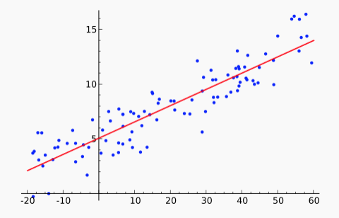
Linear regression is the process of fitting a function f to a set of (x,y) points. This is usually done by the "least squares" method: minimizing the sum of squared differences, i.e. the L2 norm. Because the error function is a simple differentiable function of the input, there is a well-known analytic solution for finding the minimum. (See the textbook or many other places.) There are also so-called "robust" methods that minimize the L1 norm (sum of absolute differences). These are a bit more complex but less sensitive to outliers (aka bad input values).

From Wikipedia

Classifier Overview

The basic set-up for a linear classifier is shown below. Look at only one class (e.g. pink for cat). Each input example generates a feature vector (x). The four pixel values $x_1, x_2, x_3, x_4$ are multiplied by the weights for that class (e.g. the pink cells) to produce a score for that class. A bias term (b) is added to produce the weighted sum $w_1 x_1 + .... w_n x_n + b$.

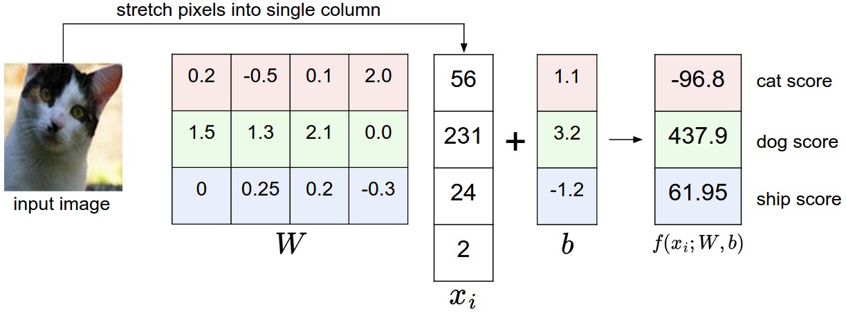
(from Andrej Karpathy cs231n course notes via Lana Lazebnik)

In this toy example, the input features are are individual pixel values. In a real working system, they would probably be something more sophisticated, such as SIFT features or the output of an early stage of neural processing. In a text classifcation task, one might use word or bigram probabilities.

To make a decision, we compare the weighted sum to a threshold. The bias term adjusts the output so that we can use a standard threshold: 0 for neural nets and 0.5 for logistic regression. (We'll assume we want 0 in what follows.) In situations where the bias term is notationally inconvenient, we can make it disappear (superficially) by introducing a new input feature $x_0$ which is tied to the constant 1 and replacing the bias term with a new weight $w_0$.

It's possible that our input data is "linearly separable," i.e. we can draw a line with all inputs of one type (e.g. cats) on one side and all inputs of the other type (non-cats) on the other. More often, there is some mixing of data points near the boundary, so the best linear boundary will leave some points on the wrong side.

Neuron Picture

We can make this process look more like a neuron or a circuit component by drawing it as follows:

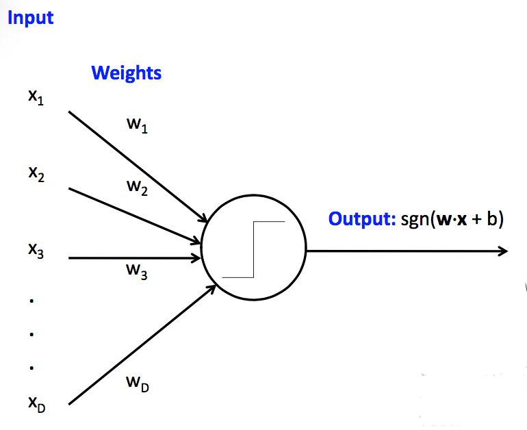(from Mark Hasegawa-Johnson, CS 440, Spring 2018)

Notice that the output is passed through the sign (sgn) function at the end. This gives us a single function $f(x) = sgn(w_1 x_1 + .... w_n x_n + b)$ which returns one of two values (1 and -1) indicating our decision (e.g. cat or not cat). We'll follow the neural net terminology and call this final function the "activation function."

Activation functions

There are a number of standard choices for the activation function, including:

• sign
• logistic(x) (also called a sigmoid) $\frac{1}{(1+e^{-x})}$
• tanh (see below)
• rectified linear unit (ReLU): f(x) = x when positive, f(x) = 0 if negative

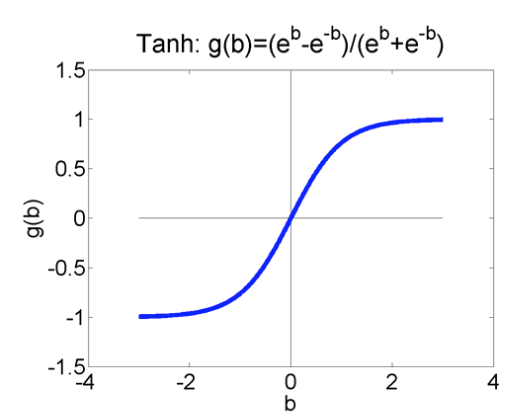(from Mark Hasegawa-Johnson)

The logistic and tanh functions are essentially the same, except that tanh returns values between -1 and 1, where the logistic returns values between 0 and 1. Wikipedia has an excessively comprehensive list of alternatives.

The activation does not affect the decision from our single, pre-trained unit. Rather, the choice has two less obvious consequences:

• The output of the logistic function is in the right range to be interpreted as a probability, if that is desired.
• A slow transition across the decision boundarie lets us treat values near the decision boundary as uncertain, both when training our unit and when feeding its value to later processing (e.g. in a neural net).

What are the weights good for?

In naive Bayes, we feed a feature vector into a very similar equation (esp. if you think about everything in log space). What's different here?

In naive Bayes, we assumed that features were conditionally independent, given the class label. This may be a reasonable approximation for some sets of features, but it's frequently wrong enough to cause problems. For example, in a bag of words model, "San" and "Francisco" do not occur independently even if you know that the type of text is "restaurant reviews." Logistic regression (a natural upgrade for naive Bayes) allows us to handle features that may be correlated. For example, the individual weights for "San" and "Francisco" can be adjusted so that the pair's overall contribution is more like that of a single word.

The training process

So far, we've assumed that the weights $w_1,\ldots, w_n$ and the bias term were given to us by magic. In practice, they are learned from training data.

Suppose that we have a set T of training data pairs (x,y), where x is a feature vector and y is the (correct) class label. Our training algorithm looks like:

• Initialize weights
• For each training example (x,y), update the weights to improve the changes of classifying x correctly.

It is common to cycle through the training examples more than once. The training algorithm would then look like this, where an "epoch" is one pass through the training data:

• Initialize weights
• For each epoch
  • For each training example (x,y), update the weights to improve the changes of classifying x correctly.

Weights can unusually be initialized to some neutral value (e.g. zero). (There are exceptions involving hidden parallel units in neural nets.)

Datasets frequently have strong local correlations, because they have been formed by concatenating sets of data (e.g. documents) that each have a strong topic focus. So it's often best to process the individual training examples in a random order.

Perceptron Learning rule

Let's suppose that our unit is a classical perceptron, i.e. our activation function is the sign function. Then we can update the weights using the "perceptron learning rule". Suppose that x is a feature vector, y is the correct class label, and y' is the class label that was computed using our current weights. Then our update rule is:

• If y' = y, do nothing.
• Otherwise $w_i = w_i + \alpha * y * x_i$

The "learning rate" constant $\alpha$ controls how quickly the update process changes in response to new data.

There's several variants of this equation, e.g.

$w_i = w_i + \alpha * (y-y') * x_i$

When trying to understand why they are equivalent, notice that the only possible values for y and y' are 1 and -1.

With this update rule, our training procedure will converge if

• data are linearly separable or
• we throttle the size of the updates as training proceeds by decreasing $\alpha$.

AI in action

Pictures illustrating how neural nets see the world. Some aspects of the world are reproduced well, but other things are seriously wrong.