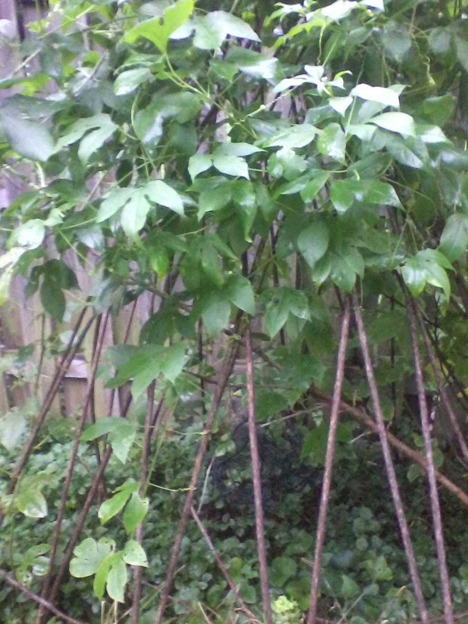
a real-world trellis (supporting a passionfruit vine)

Recap

In an HMM, we have a sequence of tags at the top. Each tag depends only on the previous tag. Each word (bottom row) depends only on the corresonding tag.

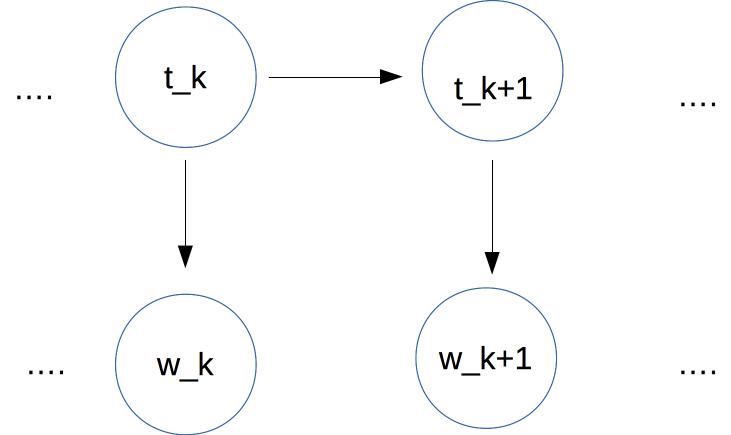
At each time position k, we assume that

\(P(w_k)\) depends only on \(P(t_k)\)
\(P(t_k) \) depends only on \(P(t_{k-1} \)

Given an input word sequence W, our goal is to find the tag sequence T that maximizes

\(P(T \mid W) \propto \prod_{i=1}^n P(w_i \mid t_i)\ \ * \ \ P(t_1)\ \ *\ \ \prod_{k=2}^n P(t_k \mid t_{k-1}) \)

So we need to estimate three types of parameters:

• \( P_I(t_1) \) initial probabilities
• \( P_T(t_k | t_{k-1}) \) transition probabilities
• \( P_E(w_i | t_i) \) emission probabilities

These are actually all just probabilities, but we're labelling them to make their roles more obvious.

Toy model

For simplicity, let's assume that we have only three tags: Noun, Verb, and Determiner (Det). Our input will contain sentences that use only those types of words, e.g.

    Det Noun     Verb    Det Noun   Noun
    The student  ate     the ramen  noodles

We can look up our initial probabilities, i.e. the probability of various values for \(t_1 \), in a table like this.

Verb	0.01
Noun	0.18
Det	0.81

We can estimate these by counting how often each tag occurs at the start of a sentence in our training data.

Transition probabilities

    Det Noun   Noun  Verb    Det Noun
    The maniac rider crashed his bike.

In the (correct) tag sequence for this sentence, the tags \(t_1\) and \(t_5\) have the same value Det. So the possibilities for the following tags (\(t_2\) and \(t_6\)) should be similar. In POS tagging, we assume that \(P_T(t_{k+1} \mid t_k)\) depends only on the identities of \(t_{k+1}\) and \( t_k\), not on their time position k. (This is a common assumption for Markov models.)

This is not an entirely safe assumption. Noun phrases early in a sentence are systematically different from those toward the end. The early ones are more likely to be pronouns; the later ones more likely to contain nouns that are new to the conversation. However, abstracting away from time position is a very useful simplifying assumption which allows us to estimate parameters with realistic amounts of training data.

Therefore, to find a transition probability \( P_T(t_k | t_{k-1}) \), we look up \(P_T(tag_a | tag_b)\) in a table like this

	\(t_{k+1}\)
\(t_k\)	Verb	Noun	Det
Verb	0.02	0.21	0.77
Noun	0.51	0.44	0.05
Det	\(\approx 0 \)	0.99	0.01

We can estimate these by counting how often a 2-tag sequence (e.g. Det Noun) occurs and dividing by how often the first tag (e.g. Det) occurs.

Notice the near-zero probability of a transition from Det to Verb. If this is actually zero in our training data, do we want to use smoothing to fill in a non-zero number? Probably yes, because even "impossible" transitions may occur in real data due to typos.

Finite-state automaton

We can view the transitions between tags as a finite-state automaton (FSA). The numbers on each arc is the probability of that transition happening.

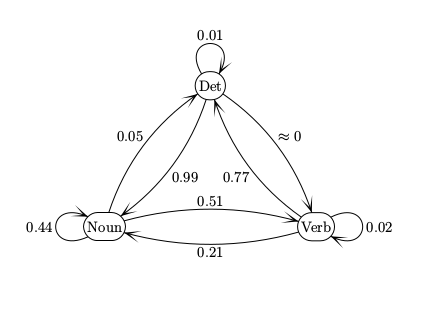
These are conceptually the same as the FSA's found in CS theory courses. But beware of small differences in conventions.

• You can start in any state (probability given by the initial probability table).
• A transition always exists between every pair of states, but each transition has an associated probability of happening.
• Output (words) is generated when you enter a state, not on the transition between states.

Emission probabilities

Our final set of parameters are the emission probabilities, i.e. P_E(word | tag). Suppose we have a very small vocabulary of nouns and verbs to go with our toy model. Then we might have probabilities like

   Verb   played 0.01
          ate   0.05
          wrote 0.05
          saw   0.03
          said  0.03
          tree  0.001
      
   Noun  boy   0.01
         girl  0.01
         cat   0.02
         ball  0.01
         tree  0.01
         saw   0.01

   Det  a    0.4
        the  0.4
        some 0.02
        many 0.02

Because real vocabularies are very large, it's common to see new words in test data. So it's essential to smooth, i.e. reserve some of each tag's probability for

• new words
• familiar words seen with a new tag

However, the details may need to depend on the type of tag Tags divide (approximately) into two types

• open class, aka content words (e.g. verbs, nouns, adjectives)
• closed class, aka function words (e.g. prepositions, determiners)

It's very common to see new open-class words. In English, new open-class tags for existing words are also likely, because nouns are often repurposed as verbs, and vice versa. E.g. the proper name MacGyver spawned a verb, based on the improvisational skills of the TV character with that name. It's much less common to encounter new closed-class words.

Decoding

Once we have estimated the model parameters, the Viterbi algorithm finds the highest-probability tag sequence for each input word sequence. Suppose that our input word sequence is \(w_1,\ldots w_n\).

The basic data structure is an n by m array, where n is the number of words in the inpuut and m is the number of different tags. Each cell (k,t) in the array contains the probability v(k,t) of the best sequence of tags for times 1-k that ends with tag t. This data structure is called a "trellis."

The Viterbi algorithm fills the trellis from left to right.

Initialization: We fill the first column using the initial probabilities. Specifically, the cell for tag t gets the value \( v(1,t) = P_I (t) * P_E(w_1 \mid t) \).

Moving forwards in time: Suppose that we have values for all tags at time k, so we need to fill in a value for each tag at time k+1. A path ending in some specific tag at time k might continue to any one of the possible tags at time k+1. So we have to consider all of these connections:

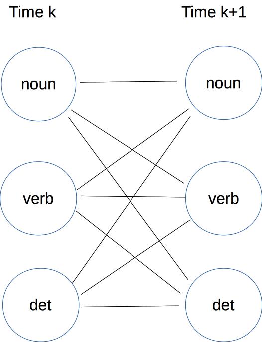
The name "trellis" comes from this dense pattern of connections between each timestep and the next.

Consider some specific tag \(tag_a\) at time k and another specific tag \(tag_b\) at time k+1. The trellis cell \( (k,tag_a)\) contains \(v(k,tag_a)\), which is the probability of the best path ending at \(tag_a\). The probability of that path continued on to \(tag_b\) is

\( v(k,tag_a) * P_T(tag_b \mid tag_a) * P_E(w_{k+1} \mid tag_b) \)

For each tag \(tag_b\) at time k+1, we compute this value for all possible tags \(tag_a\) at time k. The best (i.e. biggest) value is stored as v(k,tag_b)

Finishing: When we've filled the entire trellis, we examine the cells in the final (time=n) column and pick the one with the best (aka highest) probability.

More details

At the end of the algorithm, we need to return the best tag sequence. To do this, each cell C in the trellis must store a pointer to the previous cell that yielded best path (highest probability) to C. When you fill out the trellis to the last word, find the cell in the last column with the best value and trace backwards from it.

The probabilities get very small, creating a real possibility of underflow. So convert to logs and replace multiplication with addition.

After the switch to addition, the Viterbi computation looks a lot like edit distane or maze search. That is, each cell contains the cost of the best path from the start to our current timestep. As we move to the next timestep, we're adding some additional cost to the path. The main differences from edit distance or maze search are:

• our work is organized by the progression of time
• we prefer larger, not smaller, values

The asymptotic running time for this algorithm is \( O(m^2 n) \) where n is the number of input words and m is the number of different tags. In typical use, n would be very large (the length of our test set) and m fairly small (e.g. 40 tags in the Penn treebank). Moreover, the computation is quite simple, so ends up with good constants and therefore a fast running time in practice.

Extensions

It's worth being aware of two extensions, though we won't be covering them in detail.

• The method can be extended to use two tags of context to predict each new tag. In this case, the \(m^2\) factor becomes problematic. One would typically use beam search, i.e. keep only the most promising few paths ending at each timestep.
• Suppose that we have only very limited amounts of tagged training data, so that our estimated model parameters are not very accurate. We can use untagged training data to refine the model parameters, using a technique called the forward-backward (or Baum-Welch) algorithm. This is an application of a general method called "Expectation Maximization" (EM) and it iteratively tunes the HMM's parameters so as to improve the computed likelihood of the training data.

AI in action

Convert any line drawing into a cat (side-effect of research from Alyosha Efros's group).