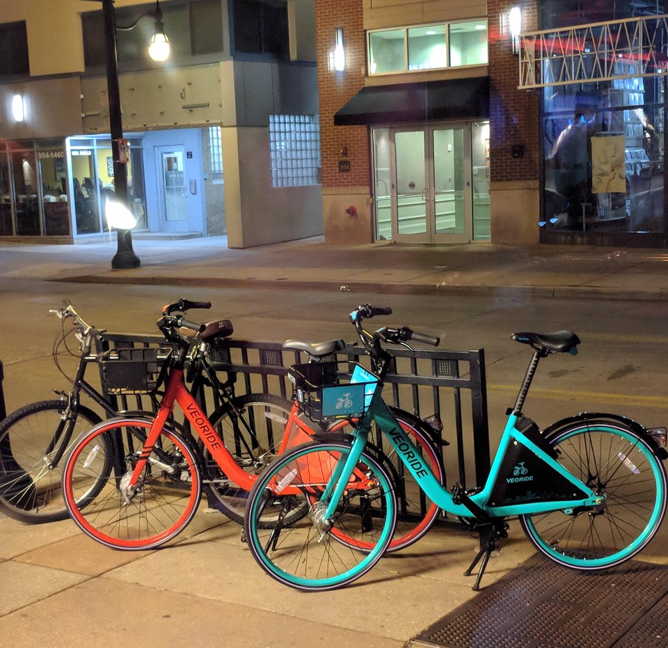
Red and teal veoride bikes from /u/civicsquid reddit post

Example: campus bikes

We have two types of bike (veoride and standard). Veorides are mostly teal (with a few exceptions), but other bikes rarely are. For simplicity, let's assume all standard (aka privately owned) bikes are red.

Joint distribution for these two variables

                 veoride        standard     |
    teal            0.19          0.02       |   0.21
    red             0.01          0.78       |   0.79
                 ----------------------------
                    0.20          0.80

For this toy example, we can fill out the joint distribution table. However, when we have more variables (typical of AI problems), this isn't practical. The joint distribution contains

• too many probability values to estimate
• too many probability values to store

Recap: conditional probability

P(A | B) is probability of A given that we know B is true. E.g.

P(teal) = 0.21
P(teal | veoride) = 0.95 (19/20)

The formal definition:

P(A | B) = P(A,B)/P(B)
equivalently P(A,B) = P(B) * P(A | B)

Flipping the roles of A and B (seems like middle school but just keep reading):

P(B | A) = P(A,B)/P(A)
equivalently P(A,B) = P(A) * P(B | A)

Bayes Rule

So we have

P(A) * P(B | A) = P(A,B) = P(B) * P(A | B)

So

P(A) * P(B | A) = P(B) * P(A | B)

So we have Bayes rule

P(B | A) = P(A | B) * P(B) / P(A)

Here's how to think about the pieces of this formula

       P(cause | evidence) =  P(evidence | cause) *  P(cause) / P(evidence)
         posterior            likelihood             prior     normalization

The normalization doesn't have a proper name because we'll typically organize our computation so as to eliminate it.

Example: we see a teal bike. What is the chance that it's a veoride? We know

P(teal | veoride) = 0.95 [likelihood]
P(veoride) = 0.20 [prior]
P(teal) = 0.21 [normalization]

P(veoride | teal) = 0.95 x 0.2 / 0.21 = 0.19/0.21 = 0.905

Why will this be useful?

In non-toy examples, it will be easier to get estimates for P(evidence | cause) than direct estimates for P(cause | evidence).

P(evidence | cause) tends to be stable, because it is due to some underlying mechanism. In this example, veoride likes teal and regular bike owners don't. In a disease scenario, we might be looking at the tendency of measles to cause spots, which is due to a property of the virus that is fairly stable over time.

P(cause | evidence) is less stable, because it depends on the set of possible causes and how common they are right now.

For example, suppose veoride's market share took a horrible drop to 2%. Then we might have the following joint distribution. Now a teal bike is more likely to be standard rather than veoride.

                 veoride        standard     |
    teal            0.019          0.025     |   0.044
    red             0.001          0.955     |   0.956
                 ----------------------------
                    0.02           0.98

Dividing P(cause | evidence) into P(evidence | cause) and P(cause) allows us to easily adjust for changes in P(cause).

The MAP estimate

Example: We have two underlying types of bikes: veoride and standard We observe a teal bike. What type should we guess that it is?

"Maximum a posteriori" (MAP) estimate

pick the type X such that P(X | evidence) is highest

Or, we should pick X from a set of types T such that

$X = \arg\!\max_{x \in T} P(x | \text{evidence})$

The argmax operator iterates through a series of values for the dummy variable (x in this case). When it determines the maximum value for the quantity (P(x | evidence) in this example), it returns the input x that produced that maximum value.

Completing our example, we compute two posterior probabilities. :

P(veoride | teal) = 0.905
P(standard | teal) = 0.095

The first probability is bigger, so we guess that it's a veoride. Notice that these two numbers add up to 1, as probabilities should.

Ignoring the normalizing factor

P(evidence) can usually be factored out of these equations, because we are only trying to determine the relative probabilities. For the MAP estimate, in fact, we are only trying to find the largest probability. In our equation

P(cause | evidence) = P(evidence | cause) * P(cause) / P(evidence)

P(evidence) is the same for all the causes we are considering. Said another way, P(evidence) is the probability that we would see this evidence if we did a lot of observations. But our current situation is that we've actually seen this particular evidence and we don't really care if we're analyzing a common or unusual situation.

So Bayesian estimation often works with the equation

P(cause | evidence) $\propto$ P(evidence | cause) * P(cause)

where we know (but may not always say) that the normalizing constant is the same across various such quantities.

Specifically, for our example

P(veoride | teal) = P(teal | veoride) * P(veoride) / P(teal)
P(standard | teal) = P(teal | standard) * P(standard) / P(teal)

P(teal) is the same in both quantities. So we can remove it, giving us

P(veoride | teal) $\propto$ P(teal | veoride) * P(veoride) = 0.95 * 0.2 = 0.19
P(standard | teal) $\propto$ P(teal | standard) * P(standard) = 0.025 * 0.8 = 0.02

So veoride is the MAP choice, and we never needed to know P(teal). Notice that the two numbers (0.19 and 0.02) don't add up to 1. So they aren't probabilities, even though their ratio is the ratio of the probabilities we're interested in.

Effect of the prior

As we saw above, our joint probabilities depend on the relative frequencies of the two underlying causes/types. Our MAP estimate reflects this by including the prior probability.

If we know that all causes are equally likely, or we have no way to estimate the prior, we can set all P(cause) to the same value for all causes. In that case

P(cause | evidence) $\propto$ P(evidence | cause)

So we can pick the cause that maximizes P(evidence | cause). This is called the "Maximum Likelihood Estimate" (MLE). It can be very inaccurate if the prior probabilities of different causes are very different.

Segue: but what if we can observe multiple types of evidence?

Suppose we are building a more complete recognition system. It might observe (e.g. with its camera) features like:

• where the bike is parked
• whether it has a kickstand.
• whether it has a filled triangular part

How do we combine these types of evidence into one decision?

Independence

Two evxents A and B are independent iff

P(A,B) = P(A) * P(B)

Equivalently

P(A | B) = P(A)

which is equivalent to

P(B | A) = P(B)

Exercise for the reader: why are these three equations all equivalent? Hint: use definition of conditional probability and/or Bayes rule. Figure this out for yourself, because it will help you become familiar with the definitions.

Sadly, independence rarely holds.

Conditional independence

A more useful notion is conditional independence. That is, are two variables independent when we're in some limited context. Formally, two events A and B are conditionally independent given event C iff

P(A, B | C) = P(A|C) * P(B|C)

Equvalently

P(A | B,C) = P(A | C)

or equivalently

P(B | A,C) = P(B | C)

Conditional independence is often a good approximation to the truth.

Basic Naive Bayes model

Suppose we're observing two types of evidence S and T related to cause C. So we have

P(C | S,T) $\propto$ P(S,T | C) * P(C)

Suppose that S and T are conditionally independent given C. Then

P(S, T | C) = P(S|C) * P(T|C)

Substituting, we get

P(C | S,T) $\propto$ P(S|C) * P(T|C) * P(C)

So we can estimate the relationship to the cause separately for each type of evidence, then combine these pieces of information to get our MAP estimate. This means we don't have to estimate (i.e. from observational data) as many numbers.

AI in action

The elephant in the room (fooling a neural net recognition system).