Tree Shaped Dynamic Programming

We’re going to look at two dynamic programming examples that both features rooted trees either in their output or input.

Woodcutting

Suppose we’re given a very long plank of wood that we need to cut up to complete some project. It’s been marked at n - 1 locations, and if we cut at all of them, we’ll get the n pieces we need for our project. Unfortunately, the only saw we know of is owned by a company with an unusual payment scheme: They charge a flat rate of $1 per foot to cut a single plank at one location, and that means we’ll have to hand back over the smaller pieces of already cut plank to do additional cuts. We need to find the cheapest way to cut up our original plank

For example, suppose n = 4, and we have marks placed at 2 feet, 3 feet, and 6 feet from the left end of the plank.

We could try cutting the marks in order from left to right, but it would cost 10 + 8 + 7 = 25 dollars, because we’d have to keep handing over the entire remaining “suffix” of our plank for each additional cut.

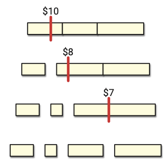
Or maybe we try the cut in the middle and then do the other two in either order. Now the total cost is 10 + 3 + 7 = 20 dollars.

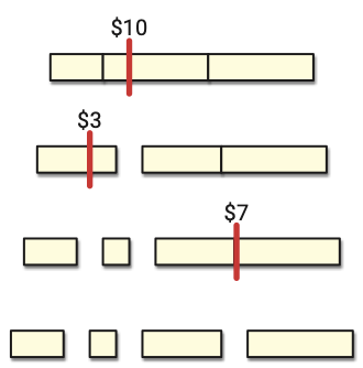
However, the best choice for these particular cut marks is to cut the positions in order from right to left at total cost 10 + 6 + 3 = 19.

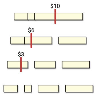
To generalize, let \mathit{Len}[1~..~n] be an array of positive numbers where \mathit{Len}[i] is the desired length of the ith board. In our example, we had n = 4 and \mathit{Len} = [2, 1, 3, 4]. How do we minimize the total cost?

I think the above figures almost give it away. Once we decide on the location for our first cut, we end up with two “subplanks” that will each get their own cuts, and best choice of cuts for the two subplanks are completely independent. If we know which is the best first cut, then the minimum cost ends up being the cost of the original plank, plus the minimum cost to cut the left subplank, plus the minimum cost to cut the right subplank. We recurse twice! Of course, we don’t know ahead of time where that best first cut is, so we’ll try all n - 1 options, doing both recursive calls corresponding to each option.

It might help to think of this process as us building a binary tree. The leaves are the final pieces of plank we desire. Our decision is where to divide the left-to-right sequence of leaves into two subtrees.

You might think this would lead to too many subproblems. Maybe one per subset of leaves or one per subsequence of \mathit{Len}. However, these subproblems represent a single connected subplank that needs to be cut up recursively. It’s an interval of the original plank that can be distinguished by two cut marks or indices of \mathit{Len}.

For any indices i \leq k, let \mathit{Cutting}(i, k) denote the minimum total cost to decompose a subplank consisting of pieces with lengths in \mathit{Len}[i~..~k]. Our ultimate task is to compute \mathit{Cutting}(1, n).

Based on the observations above, \mathit{Cutting}(1, n) obeys the following recurrence. The sum is there to get the total length of the subplank, and the min is there to help us guess the first piece we want to obtain from the right side of the cut. \mathit{Cutting}(i, k) = \begin{cases} 0 & \text{if $i = k$} \\ \sum_{j = i}^k \mathit{Len}[j] + \min\limits_{i < r \leq k} \left\{\begin{gathered} \mathit{Cutting}(i, r - 1) \\ \quad + \mathit{Cutting}(r, k) \end{gathered}\right\} & \text{otherwise} \end{cases}

Memoization

Before we do the memoization for the \mathit{Cutting} recurrence itself, let’s get rid of that summation—not because it’s actually going to save us time todo so. It’s just ugly. For any pair of indices i \leq k, let \mathit{TotLen}(i, k) := \sum_{j = 1}^k \mathit{Len}[j]. We can compute all O(n^2) values of this function using dynamic programming. Here’s the pseudocode.

Now we can more simply write our \mathit{Cutting} recurrence as \mathit{Cutting}(i, k) = \begin{cases} 0 & \text{if $i = k$} \\ \mathit{TotLen}[i, k] + \min\limits_{i < r \leq k} \left\{\begin{gathered} \mathit{Cutting}(i, r - 1) \\ \quad + \mathit{Cutting}(r, k) \end{gathered}\right\} & \text{otherwise} \end{cases}

It’s time to go through the steps.

Subproblems

The input to each subproblem for \mathit{Cutting} is two indices i \leq k specifying a subarray of \mathit{Len}[1~..~n], so 1 \leq i \leq k \leq n.

Memoization

So we’ll use a 2D array \mathit{Cutting}[1~..~n, 1~..~n]. Yes, we’ll end up ignoring all the entires in the lower left diagonal. Whatever.

Dependencies

Each entry \mathit{Cutting}[i, k] depends upon all entries \mathit{Cutting}[i, r - 1] with i < r \leq k along with all entries \mathit{Cutting}[r, k] with i < r \leq k.

Evaluation order

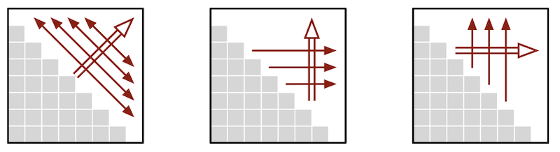
There are many different orderings we could try. Somehow the idea to try going diagonal by diagonal comes up, so why not? Let’s see what it would look like. There’s also decreasing i and increasing k nested either way.

Running time

Each call to \text{ComputeMinCost} takes O(n) time and we do O(n^2) calls for O(n^3) time total.

TODO: Pseudocode

Maximum independent set in trees

Now for a problem that looks pretty different. Given a graph G = (V, E), an independent set is a subset S \subseteq V of vertices such that no two vertices in S share an edge. We’d like to solve the following problem: Given G, what is the maximum size of any independent set? As we’ll see late in the semester, though, this problem is known to be NP-hard and very likely has no efficient algorithm.

So let’s try to make things a bit easier on ourselves. Instead of consider just any graph G, let’s consider a rooted tree T with n nodes. By definition, T has a root r, and each edge incident to r goes to the root of another, strictly smaller, rooted tree.

The recursive structure of T itself suggests a strategy we might use to solve our problem. Let’s decide whether r belongs to a large independent set S, and see what the consequences might be.

• If r \notin S, then we’re not restricting whether other nodes of T can be in S. Also, there are no edges between the subtrees of r’s children. Any independent sets in the children’s subtrees can be combined to form one big independent set of T. We can recursively ask for the maximum independent set sizes of the children subtrees and add them together.
• If r \in S, then no child of r can belong to S. However, we immediately see there’s no restriction on any grandchild subtrees. By the same reasoning as last time, we recursively ask for the maximum independent set sizes of the grandchildren subtrees and add them together (plus 1 for r itself).

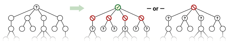
Let \mathit{MIS}(v) be the maximum size of any independent set of the subtree rooted at v. We want to compute \mathit{MIS}(r). Let w \downarrow v denote the proposition “w is a child of v” The function obeys the following recurrence: \mathit{MIS}(v) = \max \left\{\sum_{w \downarrow v} \mathit{MIS}(w), 1 + \sum_{w \downarrow v} \sum_{x \downarrow w} \mathit{MIS}(x)\right\}

Memoization

Subproblems

The input to each subproblem is a node v of the tree T.

Memoization

We’re not going to use an array this time. Instead, we’ll augment each node with an addition piece of data, storing \mathit{MIS}(v) in a new field v.\mathit{MIS}.

Dependencies

Each entry v.\mathit{MIS} depends on its strict descendants.

Evaluation order

We want to visit the nodes and compute their \mathit{MIS} values in a good order. What order guarantees we handle descendants first? A post-order traversal of T.

Running time

Here’s where the normal heuristic of (time per subproblem) x (number of subproblems) may fail. Different nodes can have vastly different numbers of children! However, we can observe that the time spend across all subproblems is proportional to the number of subproblems + the number of times we need to access all the \mathit{MIS} fields across the nodes. Each node is a child or grandchild of at most two other nodes, so we spend O(n) time total.

TODO: Pseudocode

Another approach

There’s another approach that I think is a bit less natural but ends up being a bit cleaner. We make two recurrences. Let \mathit{MISyes}(v) denote the maximum size of any independent set of the subtree rooted at v where we have to include v. Let \mathit{MISno}(v) denote the maximum size of any independent set of the subtree rooted at v where we cannot include v. We need to compute \max \left\{\mathit{MISyes}(r), \mathit{MISno}(r)\right\}. The two functions obey the following mutual recurrences. \begin{align*} \mathit{MISyes}(v) &= 1 + \sum_{w \downarrow v} \mathit{MISno}(w) \\ \mathit{MISno}(v) &= \sum_{w \downarrow v} \max \left\{\mathit{MISyes}(w), \mathit{MISno}(w)\right\} \end{align*}

The details for doing dynamic programming are essentially the same as before. We want to store subproblem solutions in two new fields on each node, and we want to compute them in postorder. The time to do so is still O(n).