Turing Machines

Escalating capabilities

In the first few weeks, we discussed regular languages, those made by combining individual strings via union, concatenation, and repetition (Kleene closure.) You might say they are “generated” by regular expressions (basically by definition.) In addition, Kleene’s theorem says regular languages are accepted by DFAs and NFAs, two machine models with a fixed finite amount of “memory”.

Our proofs that certain languages are not regular, used the fact that memory is limited. Intuitively, not having unbounded memory means our machines cannot remember what happens to arbitrary length sections of a string to place requirements upon later sections of the same string. You can also see that intuition in regular expressions: two subexpressions being concatenated together do not share any information about what strings they’re generating.

So last time, we discussed a model that gets around these limitations by including a very restrained way to share information: recursion via context-free grammars (CFGs.) The languages generated by CFGs are themselves called context-free. There are also machine models that accept the context-free languages. Erickson (5.8)[https://courses.grainger.illinois.edu/cs374al1/fa2025/notes/models/05-context-free.pdf] introduces recursive automata.¹ An hour and a half ago, Section B saw push-down automata (PDAs.)²

In recursive automata, you essentially have a finite number of NFAs where individual transitions are allowed if and only if a prefix of your input string can be accepted by recursively feeding it to one of those NFAs.

In push-down automata, you essentially have a single NFA along with a stack. Transitions are based both on the current symbol from the input string along with the symbol on the top of the stack. Each transition has the option of pushing a single symbol onto or popping a single symbol off of the stack.

The extra power from CFGs was enough to generate languages like $\{0^n 1^n \mid n \geq 0\}$ , but information shared between parts of the generated string had limitations. In particular, once you use the information (popped the stack in the case of PDAs,) you could not recover it again.

The one big thing we’re missing is unbounded memory that not only remembers what we’ve done but also can be reused or modified. Surprisingly, the introduction of this memory is enough to handle any kind of arbitary (finite) computation, and there are many many specific models for the kinds of “machines” you might base on it. Python programs that read a string and return a Boolean, a persistent individual with an unbounded quantity of paper and coffee (i.e., a tireless mathematician), and a model by Alan Turing all fit under this idea, and they all decide what strings belong to the exact same family of languages.

Capabilities	Languages	Models
Union Concatenation Repetition	Regular	Regular expresions DFAs NFAs
+ Recursion	Context-free	CFGs Recursive NFAs PDAs
+ Memory	(Decidable) (Recursive)	Arbitrary computation Python Persistent individual with unending paper and coffee (a Tireless Mathematician) Turing’s model (now called the Turing machine)

We’re going to discuss that last model, the Turing machines, but the focus will be fairly different from when we covered regular or even context free languages. What makes Turing machines interesting isn’t their specific properties or how to design them (which we won’t ask you to do directly,) but instead their history and what they tell us about the limitations of arbitrary finite computation.

History

A longstanding challenge in mathematics has been to development general methods for figuring out the truth of various statements. In particular, Hilbert and Ackermann posed the Entscheidungsproblem (German for “decision problem”) in 1928, asking if there is an algorithm that can determine if any given proposition is provable from the axioms of first-order logic.

Half the challenge in provably settling the question is in defining what “algorithm” even means. Within a few years, three ideas were presented:

Gödel proposed general recursive functions,
Church proposed the (untyped) $\lambda$ -calculus, and
Turing proposed what we now call Turing machines.

And under all three models, the answer is no, there is no algorithm for determining if a proposition is true!

Gödel’s incompleteness theorems don’t feel like a model of computation in the same way we’re used to thinking of it. Church’s is closer, and it is arguably the best was to think about program evolution or how to define the semantics of a programming language. In my opinion, however, Turing machines strike the best balance between being simple enough to formally define and reason about while also feeling like how a computer or even a human would do computations.

That said, both of the latter two models can handle the same family of languages, and they’re likely the most powerful models we have while still feeling “reasonable”. In particular, the largely believed Church-Turing thesis says that all finite computation can be modeled using the $\lambda$ -calculus or a Turing machine.

How they work

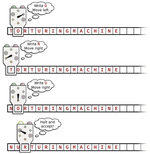
Informally, you can think of a Turing machine as modeling a human doing computation by hand with a very very very large stack of paper (and there’s always more paper available in the cabinets near the printer.) You have a machine with a finite set of internal states. Continuing with the human computer analogy, it models our brain’s limited ability to remember much of what’s going on without writing it down somewhere.

Fortunately, we can write things down. The machine has access to some “memory” in the form of an infinite tape. In the analogy, the tape models the stack of paper.

The tape contains a semi-infinite (one of the two extremes is bounded) sequence of cells, each containing a single symbol from a finite alphabet; the stack of paper is very tall but has a top sheet. The input string $w$ is initially written found in the first/leftmost $|w|$ cells. The machine can access the tape through its head which moves around during computation but can only interact with one cell at a time; we can only have one sheet as the current one that we’re looking at and writing on.

And based on the current internal state and what is written at the head’s cell, the machine changes state, writes a symbol (possibly the same as the one already there), and moves one cell to the left or right; it’s hard to shuffle between several sheets of paper at a time without losing track of what you’re doing, but it is possible to go one sheet up or down the stack.

Finally, there are two special states. If the machine ever reaches an accept state, it accepts the input string, and if it ever reaches a reject state, it rejects the input string. A few iterations of a six-state Turing machine

Formal definitions

A Turing machine consists of the following components:

A arbitrary finite set $\Gamma$ with at least two elements: the tape alphabet
An arbitrary symbol $\square \in \Gamma$ : the blank symbol
An arbitrary nonempty subset $\Sigma \subseteq (\Gamma \setminus \{\square\})$ : the input alphabet
An arbitrary finite set $Q$ : the states
Three distinct special states start, accept, and reject $\in Q$
The transition function $\delta: (Q \setminus \{\textbf{accept}, \textbf{reject}\}) \times \Gamma \to Q \times \Gamma \times \{-1, +1\}$

Yes, it’s a lot. The exact behavior of the machine can be described as follows. At all times, the machine is in a configuration $(q, x, i) \in Q \times \Gamma^* \times \mathbb{N}$ . This configuration represents:

being in internal state $q \in Q$ ,
with our tape holding the string $x \in \Gamma^*$ followed by an infinite sequence of blanks (i.e., $x$ is in the first/leftmmost $|x|$ cells, and all cells to its right are blank,) and
with the head of the machine located at position $i \in \mathbb{N}$ where $0$ is the position of the leftmost cell Given input string $w \in \Sigma^*$ , the machine starts in configuration $(\textbf{start}, w, 0)$ .

At each step, the machine applies the transition function to change configuration. Suppose the machine is in configuration $(p, xay, i)$ with $|x| = i$ (i.e., the head is pointed at the cell containing $a$ .) The machine uses its current state $p$ and the symbol $a$ under the head to determine what to do. If $\delta(p, a) = (q, b, +1)$ , then the machines moves to configuration $(q, xby, i + 1)$ , and if $\delta(p, a) = (q, b, -1)$ , then the machines moves to configuration $(q, xby, i - 1)$ . In other words, it goes to an internal state according to the first component of $\delta(p, a)$ , while writing a symbol in place of the $a$ according to the second component of $\delta(p, a)$ , and moving the head one position left or right according to the third component.

The machine immediately accepts $w$ if (after a finite number of transitions) it reaches internal state accept, and it rejects $w$ if it reaches internal state reject.

Those are not the only two possible results! The machine might crash by moving the head to position $-1$ . We generally don’t worry about whether a Turing machine crashes; if it’s designed well, it shouldn’t happen. And as we’ll see shortly, the possibility of crashing does not grant any additional power or what the machine is capable of. From here on, I’ll write as if a machine never crashes.

Even with the above stipulation, it’s still possible that a Turing machine never reaches an accept or reject state. In particular, lack of acceptance does not imply rejection³ If the machine does not accept, reject, or crash on $w$ , then we say it diverges.

Do not take this as life advice. I am not a therapist.

A Turing machine diverges or fails to halt on $w$ if it does not accept or reject on $w$ . It halts on $w$ if it accepts or rejects.

There are now more than two possibilities with what happens to an input string, so it makes sense to discuss multiple languages for a Turing machine. Let $M$ be a Turing machine. We define the following four languages: $\begin{align*} \text{Accept}(M) &:= \{w \in \Sigma^* \mid \text{$M$ accepts $w$}\} \\ \text{Reject}(M) &:= \{w \in \Sigma^* \mid \text{$M$ rejects $w$}\} \\ \text{Halt}(M) &:= \text{Accept}(M) \cup \text{Reject}(M) \\ \text{Diverge}(M) &:= \Sigma^* \setminus \text{Halt}(M) \end{align*}$

We say $M$ accepts or recognizes $\text{Accept}(M)$ I’ll stick to the term accepts. Similarly, $M$ rejects $\text{Reject}(M)$ . It halts on $\text{Halt}(M)$ and diverges on $\text{Diverge}(M)$ .

Language $L$ is acceptable or recursively enumerable or recognizable or semi-computable if some Turning machine accepts $L$ , i.e., there exists a machine $M$ such that $L = \text{Accept}(M)$ . I’ll tend to stick to acceptable for this class, even though the term is not terribly common. For reasons we won’t go into, recursively enumerable is the term you’re most likely to encounter outside of this class.

If language $L$ is acceptable, then there exists a Turing machine that is guaranteed to accept exactly the strings in $L$ , but it may run forever on strings outside of $L$ , meaning the machine itself may try and try and try to check for inclusion in $L$ and we’ll never know if it should just give up. It’s like a mathematician trying every possible proof of a statement without knowing if a proof exists.

In many cases, however, one can figure out (after a finite amount of time) whether a string does or does not belong to a language. Turing machine $M$ decides language $L$ if it accepts every string in $L$ and actually rejects every string in $\Sigma^* \setminus L$ ( $L = \text{Accept}(M)$ and $\bar{L} = \text{Reject}(M)$ .) Equivalently, $M$ decides $L$ if $M$ accepts $L$ and it always halts ( $L = \text{Accept}(M)$ and $\Sigma^* = \text{Halt}(M)$ .) $L$ is decidable or recursive or computable if it is decided by some Turing machine. Decidable is the most commonly used term in and out of this class, although recursive might come up in contexts where recursively enumerable comes up.

Every decidable language is acceptable (by definition,) but the surprising thing is that there are acceptable languages that are not decidable. Showing this claim was a key part of Turing’s insights, but we won’t be able to fully appreciate this fact until much later in the semester.

Our one example

Again, we’re not going to ask you design Turing machines in any assignments or exams. It’s incredibly tedious to do, and most of the value in Turing machines (for this class at least) is about seeing what a sufficiently powerful model of computation is capable of. We’ll look at one example for completeness, though.

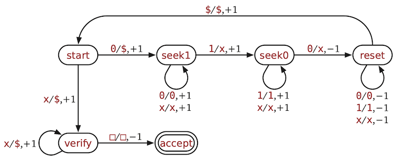
Consider the canonical noncontext-free language $L = \{0^n1^n0^n \mid n > 0\}$ . It is decided using a Turing machine with a mere six states.

$\Gamma = \{0, 1, \$, x, \square\}$
$\Sigma = \{0, 1\}$
$Q = \{\text{start}, \text{seek1}, \text{seek0}, \text{reset}, \text{verify}, \text{accept}, \text{reject}\}$

The transitions are described using the following transition graph. The label $a/b,z$ on an edge $p \to q$ means $\delta(p, a) = (q, b, z)$ . Missing transitions go to $\text{reject}$ . The transition graph for a Turing machine deciding 0^n1^n0^n To summarize,

The machine repeatedly scans the input string from left to right marking the first unmarked 0, then 1, then 0 it sees with a $, an $x$ , and an $x$ , respectively. It then resets the head back to the rightmost $ and repeats the process.
The repetitions end when the machine either fails to encounter an expected symbol during a pass (leading to immediate rejection), or the rightmost $ occurs just before the first $x$ .
It then makes sure that every non-blank symbol after the rightmost $ is an $x$ as proof that neither the second nor third run was longer than the first.
If it’s gotten this far, it can safely accept.

There’s a trace of how the configuration changes in Erickson’s notes (which may have a typo?) but yuck!

All finite computation

The Church-Turing thesis states that Turing machines can model any computation by finite means. In principle we can’t prove the thesis (we’d need to define computation and uh… that’s kind of the point of defining Turing machines.) In particular, all reasonable variations on Turing machine that might seem more powerful (or convenient) can be simulated by a Turing machine as described above. We’ll not go over detailed arguments, but here are some examples.

Doubly infinite tapes (with negative positions.) Now we avoid crashing!
Multiple tapes, each with their own head that can move independently of the others even as all the heads are used to decide what each transition should do. This extension is useful for studying space usage as something distinct from the length of the input string.
Non-determinism. At each transition, you get to pick from a finite number of options for how to proceed. If any sequence of choices reaches the accept state, you accept the string.

Turing machines can also model programming paradigms that you might be used to (albeit with a worse running time) such as

loops,
function calls,
pointers/references, and
arrays.

They can even model the concept of programming and program interpretation. Every Turing machine has a finite tape alphabet and a finite set of states, so every Turing machine $M$ can be fully described using a finite string we’ll denote as $\langle M \rangle$ . Similar to how we can write a Python interpreter in Python, there exists something called the universal Turing machine $U$ . It that takes a string $(\langle M \rangle, w)$ encoding another Turing machine $M$ and an input string $w$ for $M$ . Then,

$U$ accepts $(\langle M \rangle, w)$ if and only if $M$ accepts $w$ , and
$U$ rejects $(\langle M \rangle, w)$ if and only if $M$ rejects $w$ . Erickson’s book describes one way to encode the string $\langle M \rangle$ and the machine $U$ itself.

The idea that any sufficiently advanced model of computation can model itself was one of Turing’s key insights. As we’ll see late in the semester, this property of computation can be used to explain why the Entscheidungsproblem has a negative answer and why there are acceptable languages that are not decidable.