Shortest Paths (Preferably With Positive Edge Weights)

We’ll return to dags and dynamic programming soon, but first, we’ll build motivation for a problem we’d like to solve with them.

We’re given a directed graph G = (V, E) with edge weights w: E \to R and a single vertex s \in V. We want to compute the the shortest path from s to some vertex, and it turns out almost all algorithms for doing so actually compute the shortest paths from s to (nearly) all other vertices. We’re solving the single source shortest path (SSSP) problem.

For this lecture, we’ll assume edges weights are positive. These paths have a nice structure in that we may assume they never diverge and meet again. For example here:

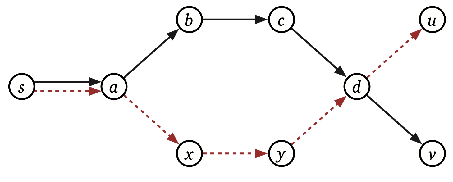
If both the black solid and red dotted paths are shortest for their respective targets, we can redirect one to stick to the other and not diverge. Here, we’d replace a \to x \to y \to d with a \to b \to c \to d. And therefore, we may assume all the shortest paths out of s form a shortest path tree rooted at s.

FordSSSP

Nearly all algorithms for SSSP follow the a single framework first proposed by Lester Ford in 1956. We maintain two values for each vertex v:

• v.\textit{dist} is the length of some tentative path from s to v (or \infty if we’ve yet to find such a path)
• v.\textit{pred} is the predecessor of v in the tentative path of length v.\mathit{dist} (or Null if v.\mathit{dist} = \infty) Note that following \mathit{pred} pointers does not necessarily give us a path of length v.\mathit{pred} at all times. All we know for sure is that there exists some path ending in v.\mathit{pred} \to v of length v.\mathit{dist}. It’s possible that the \mathit{pred} pointers further back in the path have themselves been updated so following them gives a shorter path implied by some v.\mathit{dist}.

At first, we only know of one path, the trivial one from s to itself, and as far as we know, there are no paths from s to any other vertex v \neq s. We initialize the \mathit{dist} and \mathit{pred} values accordingly.

How do we find better paths to other vertices? We look for tense edges. An edge u \to v is tense if u.\mathit{dist} + w(u \to v) < v.\mathit{dist}. We’re observing that our tentative path to v can’t be the shortest one, because the tentative path to u followed by u \to v is shorter. We deal with tense edges by relaxing them as follows:

Now, the tentative path to v is the one that follows the tentative path to u and then follows u \to v. Much better.

Ford’s strategy is to repeatedly relax tense edges until no more remain.

Lemma: Assuming G has non-negative edges weights, \text{FordSSSP}(s) will terminate with all v.\mathit{dist} set to the distance from s to v and all v.\mathit{pred} set to the predecessor of a shortest path from s to v.

I’m not going to attempt to give the full proof here or in lecture. In addition to what’s written above about each v.\mathit{dist} values always being the length of some (s, v)-path and v.\mathit{pred} values always being the predecessor on that path, I’d need to argue that if any of the \mathit{dist} values are too high, there’s at least one on the far side of a tense edge. We can always find a tense edge until the distances and predecessors are found, and because each change to some v.\mathit{dist} refers to the length of a path to v never found before, we’ll eventually run out of better and better paths to work with, resulting in the algorithm terminating for sure.

However, there might be a lot of paths from s to any one vertex v. Our goal for this lecture and the next one is to be clever in how we pick tense edges to relax so the total number of relaxations is relatively small. All shortest paths algorithms we’ll discuss can be thought of in this framework. Similar to running WhateverFirstSearch with different bags, each shortest paths algorithm is based on use picking tense edges in a different order. The specific order we want to use depends heavily on both the weights of the edges and the structure of the graph.

Arbitrary non-negative weights: best-first

Again, we’re assuming for this lecture that edges weights are arbitrary positive real numbers. The best algorithm for this case was independently discovered many times over, but it’s most commonly attributed to Dijkstra today.

We’re going to consider a variant of Dijkstra’s algorithm that (in my opinion) better captures the goals of the FordSSSP framework and has another benefit we’ll get to shortly. It’s based on a couple observations:

• If edge u \to v is not tense, then it cannot go tense until u.\mathit{dist} decreases. In particular, an incidental decrease to v.\mathit{dist} can only help the edge feel more relaxed.
• Let u \to v be a tense edge that minimizes u.\mathit{dist}. We may assume u.\mathit{dist} is already the distance from s to u, so we should prioritize such edges over others. I’ll say a bit more on why this observation is true later.

In this pseudocode, we’re using a priority queue where Insert takes first an object and second its priority. The DecreaseKey operation can be used to decrease the priority of an object. The ExtractMin operation extracts the object with minimum priority.

Observe how the priority is always set to the current value of v.\mathit{dist}.

We can imagine the algorithm computing computing distances according to an outgoing wavefront from s.

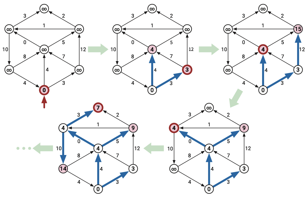
So, is it correct, and is it fast? I’ll speak to correctness first. As mentioned above, the priority queue contains all vertices at the tail/beginning of every tense edge (and possibly some more). In more detail, recall that \mathit{dist} values can only decrease, and therefore an edge u \to v can only become tense if u.\textit{dist} changes. Therefore, we insert s into the priority queue right after InitSSSP, and whenever we relax an edge u \to v, we immediately put v into the priority queue if it isn’t there already. By repeatedly extracting vertices from the priority queue until we are no longer able to do so, we make sure that any tense edge is eventually examined and subsequently relaxed if it is still tense. We match the FordSSSP model and therefore find the shortest path distances eventually.

So what about running time? There’s a more formal argument in Erickson Chapter 8, but here’s the gist. Let d_i be the \mathit{dist} value of the ith vertex we extract from the priority queue. We use ExtractMin and have non-negative weights on the edges, implying each d_{i+1} \geq d_i. In short, we remove something of smaller distance than all other members of the priority queue and then do relaxations that cannot reduce the \mathit{dist} values below d_i. Each v.\mathit{dist} only decreases, and anything we put in the priority queue eventually comes back out. By the previous observation, after the first time we extract v from the priority queue, it can’t go back in again. We touch every vertex and outgoing edge at most once, so the assuming the graph is connected and simple, the running time is O(|V| + |E| \log |E| = |E| \log |V|).

Unweighted graphs: Breadth-first search

But what if the weights are not only positive but all equal to 1? You use a breadth-first search (BFS). We saw a version that fit cleanly into the WhateverFirstSearch framework. Here’s an alternative that better matches FordSSSP. Here, we have a single queue data structure supporting Push (queue) and Pull (dequeue) operations.

Again, we’re assuming right now that all weights are equal to 1 so the + 1 bits here and there are accurately checking for tenseness and doing relaxations. Correctness follows from the same argument as with Dijkstra’s algorithm: we need only add v to the data structure when v.\mathit{dist} decreases.

And then running time? It’s no longer “by design”, but like with Dijkstra’s algorithm, we always end up grabbing the minimum \mathit{dist} vertex from the queue whenever we do a Pull. To see why, assume inductively that 1) the members of the queue are sorted increasing order of \mathit{dist} value and 2) v.\mathit{dist} is equal to either the distance from s to v or \infty, and 3) the final member of the queue has \mathit{dist} at most one greater than the first member. When we relax an edge u \to v, the induction hypothesis implies v.\mathit{dist} = \infty, so v is not yet in the queue. Also, u has the minimum distance of anything that can relax v. Therefore, u.\mathit{dist} + 1 is the true distance of v. We set v.\mathit{dist} to the correct distance, which is one greater than the first member of the queue, and stick it in the back because it becomes the largest distance member.

Erickson Chapter 9 has a more visual argument where we stick a token between members of the queue that have different \mathit{dist} values. You may be interested to check it out.