Shortest Paths With Negative Edge Weights

In the last lecture, we considered the single source shortest paths (SSSP) problem: Given a directed graph G = (V, E) with real edge weights w: E \to \mathbb{R} and a single vertex s \in V, we want both the distance from s to every other vertex and the rooted tree of shortest paths out of s.

Last time, we worked under the assumption that the edge weights were positive. A special case under that assumption is that all edges weights are equal to 1. If that’s true, we should use a BFS running in O(|V| + |E|) time; however non-unit edge weights will result in BFS just being wrong. For more general positive weights, we should use Dijkstra’s algorithm. It will compute shortest paths from s in O(|E| \log |V|) time total (with that simplified running time assuming G is connected and simple). Here was the code, including its two subroutines.

Correctness followed from Dijkstra’s algorithm being a special implementation of Ford’s generic approach to solving SSSP.

There is nothing about the SSSP problem definition that requires us to assume positive edge weights, and there are (perhaps not immediately intuitive) applications for negative weights. Surprisingly, Ford’s approach can still work with negative edge weights, but with one major caveat. The problem is that FordSSSP isn’t really looking for shortest simple paths. In fact, the problem of finding shortest paths with negative edge lengths is NP-hard in general.¹ FordSSSP is really looking for shortest walks, and those might not exist in some cases.

When edge weights are positive, all shortest walks are, in fact, paths; if a walk repeats a vertex v, then the portion between the two instances of v can be removed, shortening the walk. However, if there is a path from s to a cycle C of negative weight, then for every vertex v reachable from a vertex of C, any walk from s to v can be shortened by following a walk from s to C, following C a sufficient number of times, and walking from C to v. On the other hand, there’s still no need for a short walk to follow a cycle if the cycle has non-negative weight. We’ll amend our lemma from last time:

Lemma: Assuming G has no negative weight cycles, \text{FordSSSP}(s) will terminate with all v.\mathit{dist} set to the distance from s to v and all v.\mathit{pred} set to the predecessor of a shortest path from s to v.

Once again, correctness of Dijkstra’s algorithm as given above is based on it being an implementation of FordSSSP; it still makes sure to check each edge u \to v that for tenseness every time it could possibly become tense. As long as there are no negative weight cycles, \text{Dijkstra}(s) will find all shortest paths and distances from s.²

Unlike correctness, though, the running time analysis we did does depend on edge weights being positive (or non-negative). It turns out \text{Dijkstra}(s) will continue to run quickly if there are very few negative weight edges (say, just one like in the lab problem), but if there is no limit on the number of negative weight edges, it might end up taking exponential time to finish.

The goal for this lecture is to find shortest paths with negative edge weights more quickly, assuming there are no negative weight cycles.

Dags: dynamic programming

FordSSSP suggests our only obstacle for computing shortest paths is the existence of a negative weight cycle, so let’s start with a class of graphs that we can be absolutely certain don’t have one, dags.

Recall from an earlier lecture that a recursive algorithm can only run to completion if its dependency graph is acyclic. Conversely, if the algorithm’s dependency graph is a dag, then not only will the algorithm run to completion, but we can compute an ordering of the subproblems that will be useful for memoization. Specifically, any topological ordering of the (ahem) reversal of the dependency graph will do (if the dependency graph contains u \to v, we need to complete subproblem v first).

Now, let’s go back to shortest paths in a dag G = (V, E) with weights w: E \to \mathbb{R} and source vertex s. We’re going to come up with a recursive solution to the problem where the dependency graph is also a dag. To that end, let \mathit{distance}(v) denote the distance from s to v. If the shortest path from s to v \neq s ends with edge u \to v, then it follows the shortest path from s to u and then that edge. More concisely, \mathit{distance}(v) = \begin{cases} 0 & \text{if \(v = s\)} \\ \min\limits_{u \to v} (\mathit{distance}(u) + w(u \to v)) & \text{otherwise.} \end{cases}

Again, this recurrence is usable if and only if its dependency graph is a dag, and sure enough, the dependency graph is actually (the reversal of) G itself (with some edges incident to s removed due to the base case).

How do we memoize? We wanted to compute those \mathit{dist} and \mathit{pred} values anyway, so let’s store solutions directly into \mathit{dist} (we’ll worry about \mathit{pred} later). We need to compute \mathit{distance}(u) before \mathit{distance}(v) for each edge u \to v, so we should compute them in a topological order. Finally, we spend constant time per vertex storing solutions and (across all subproblems) constant time per edge looking up already computed distances. Even counting the time to compute a topological order, the algorithm should take O(|V| + |E|) time total. Below is the pseudocode based on a straightforward implementation of the dynamic programming approach. Yes, I’m fine with not having yet another line just for computing the topological order.

We can write the code more concisely (and compute the shortest paths tree itself) by recasting it into the FordSSSP framework:

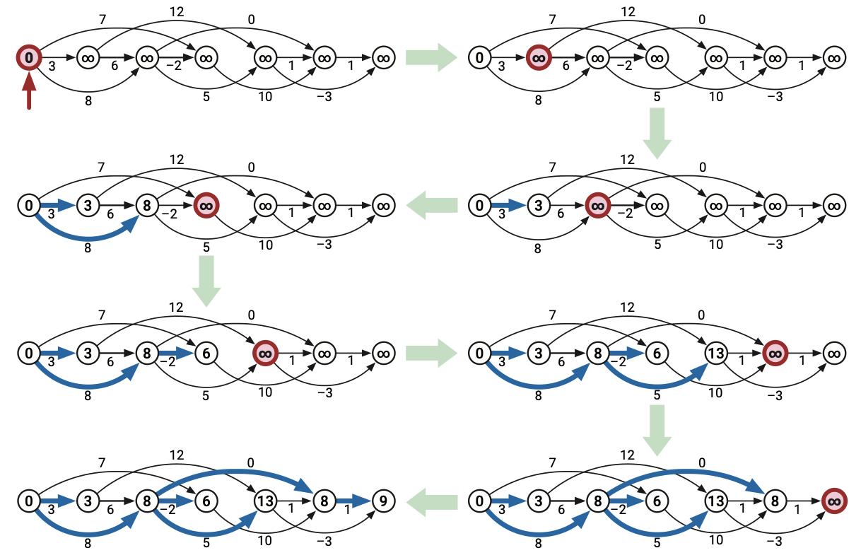
Here’s what a run of the algorithm might look like.

Aside: Dynamic programming in a dag

We just saw an example of a dynamic programming algorithm where the subproblems are based on vertices in a dag. In this case, the dependencies were based on incoming edges, so we handled the subproblems in topological order.

Sometimes, though, dependendies are based on outgoing edges. For example, let’s mix things up (and match an example in Erickson 9) by computing longest paths into a vertex t. Let \mathit{longest}(u) denote the maximum length of any path from from v to t. Then \mathit{longest}(u) = \begin{cases} 0 & \text{if \(u = t\)} \\ \max\limits_{u \to v} (w(u \to v) + \mathit{longest}(v)) & \text{otherwise.} \end{cases} In this case (and because there are no additional parameters) the input dag itself is the dependency graph. To memoize, we’d need, for each edge u \to v, to solve each subproblem v before subproblem u. We want the reversal of a topological order. And based on what we did a couple lectures ago, that means we should solve the problems in postorder.

(We could have also run DagSSSP directly on the reversal of G with negated edge weights. It’s the same algorithm.)

In a way, we’ve been doing this sort of thing the entire time we’ve been looking at dynamic programming. Even for nicely structured things like edit distance, there was an underlying dependency graph in which we needed to solve subproblems. And the way to do so is always in a postorder of the dependency graph. We just happened to pick a particularly nice looking postorder and bake it into some for loops.

When all else fails: (layered) Bellman-Ford

So what do we do if there are negative weight edges, but we don’t have a dag? Again, the situation is kind of hopeless if there are negative weight cycles, so let’s assume for now that there aren’t any.

There’s a very slick (but not particularly fast) algorithm for this case. It has variants that can be creditted to a lot of different researchers, but most people simply attribute it to Bellman and Ford. I am not going to give the true simple clean pretty version of Bellman-Ford today. Instead, we’re going to design a new algorithm that’s good enough for stating the running time bounds. We’ll see another way of thinking about it in the next lecture, and that way will lead to its most common description.

Let G = (V, E) be an arbitrary directed graph (possibly with cycles) with edge weights w: E \to \mathbb{R} and s \in V. Assuming G has no negative weight cycles, shortest walks from s do exist, and they always follow simple paths. A path in G has at most |V| vertices and |V| - 1 edges.

The main idea for this lecture is that we’re going to design an algorithm that computes, for each vertex v and each i \in \{0, \dots, |V| - 1\}, the length of the shortest walk from s to v with exactly i edges (or the value \infty if not such walk exists). We’ll do so via graph layering.

We’ll build a graph G' = (V', E') with edge weights w' : E' \to \mathbb{R} whose vertices represent reaching different vertices of G using walks with a specified number of edges. In more detail:

• V' := \left\{(v, i) \mid v \in V, i \in \{0, \dots, |V| - 1\}\right\}.
• E' := \left\{(u, i - 1) \to (v, i) \mid u \to v \in E, i \in \{1, \dots, |V| - 1\}\right\}.
• w'((u, i - 1) \to (v, i)) := w(u \to v) for all u \to v \in E and i \in \{1, \dots, |V| - 1\}.

For each vertex v, the distance from s to v in G is precisely the minimum over all i of the distance from (s, 0) to (v, i) over all i. The graph G' is a dag, because every edge only goes from lower second index to higher. Therefore, we can call DagSSSP((s, 0)) and then compute the minimum described above to get the distance to each vertex in G.

The dag G' has (|V| - 1) \cdot |V| = O(|V|^2) vertices and (|V| - 1) \cdot |E| = O(|E||V|) edges. Assuming G is simple and connected, our algorithm for shortest paths with negative edges (but no negative weight cycles) runs in O(|E||V|) time.

All that said, this new algorithm is not quite a FordSSSP variant (our final product for next time will be), but it does compute the correct distances. In fact, it computes the correct lengths of shortest walks with at most i edges even when there are negative weight cycles.

Recall the lemma what is written above about FordSSSP and negative weight cycles, though. In short, if we assign to each vertex the value v.\mathit{dist} computed above, there will still be a tense edge if and only if we have not computed the correct distances from s. The only way we haven’t computed those distances is if there is a negative weight cycle reachable from s. To conclude: we can detect if G has a negative weight cycle in O(|E||V|) time by running the above algorithm and then checking each edge to see if it is tense.

For homework and lab, you’re free to call the O(|E||V|) time shortest paths computation and negative cycle detection Bellman-Ford. You’ll see the (surprisingly slick) actual implementation of Bellman-Ford in the next lecture.

Summary of shortest paths algorithms

We’ve now gone over four algorithms for computing shortest paths in a directed graph G = (V, E). The best one to use depends upon the structure of the graph and how the edge weights are valued. Assuming G is simple and connected,

• If all weights are 1, meaning you want paths with a minimum number of edges, use BFS in O(|V| + |E|) = O(|E|) time.
• If G is a dag, use DagSSSP in O(|V| + |E| = |E|) time.
• If G is not a dag, but edge weights are positive (or even non-negative), use Dijkstra’s algorithm in O(|E| \log |V|) time.
• If none of the above apply, use Bellman-Ford in O(|E||V|) time.

Those will all be fine in theory and in practice. If all you care about is the theory, though, there has been some very recent progress.

For non-negative weights, there is an algorithm that runs in O(|E| \log^{2/3} |V|) time [DMMSY ’25]. For graphs with negative weight edges, there are a few “best” algorithms depending on exactly how |E| and |V| compare. One of them from summer 2026 is by Kent Quanrud and Navid Tajkhorshid and runs in the better of O(|E||V|^{0.7193}) and O((|E||V|)^{0.8620}). Kent is one of Chandra Chekuri’s former Ph.D. students, and (as of Fall 2026), Navid is still an undergrad at UIUC, and he is (was?) a CA for CS 225 and was a CA for CS 374 through Spring 2026.