Dynamic Programming

Virahanka (Fibonacci) numbers

There is a famous sequence of numbers that apply to many phenomena found in both nature and art. For each non-negative integer n, we let F_n := \begin{cases} 0 &\text{if $n = 0$}\\ 1 &\text{if $n = 1$}\\ F_{n - 1} + F_{n - 2} &\text{otherwise} \end{cases}

This sequence was first described by Virahanka around 800 CE while writing commentary about Pingala’s study of classical Sanskrit poetry. It was also described by Fibonacci in 1202.

Let’s say we want to compute Finonacci numbers¹ The recurrence immediately suggests a recursive algorithm for doing so.

If we try to analyze this algorithm, or even run it for moderate values of n, we’ll see that it’s horrendously slow. Up to constant factors, it follows the recurrence T(0) = 1, T(1) = 1, and T(n) = T(n - 1) + T(n - 2) + 1 for all n \geq 2. That looks like the Fibonacci recurrence again, and indeed, T(n) = 2F_{n + 1} - 1 = \Theta(\phi^n) = O(1.62^n). A quick look at the recursion tree shows what’s going wrong here. In this case, the value of each node is the number it computes.

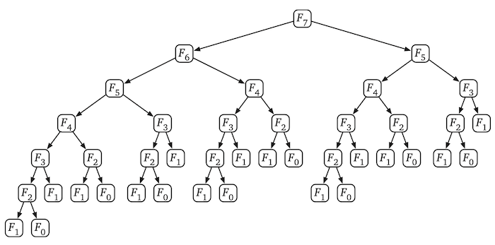
That is a lot of recursive calls. In fact, we can infer that there are exactly F_n leaves with value F_1, because that’s the only non-zero base case and they add up to F_n. Which then implies there are at least F_{n + 1} - 1 internal nodes with many many many of them with value F_2 and slightly fewer with value F_3… There is a LOT of repeated work!

Donald Michie proposed one solution to this problem in 1967 when describing how programming languages should support “memo functions” that remember the results of previous function calls. We now call adding this feature to a function “memoization”. Basic memoization uses a “global” data structure to store the return values of function calls the first time they are computed so every time after that the value can be retrieved more quickly.

So what’s a good data structure to use? We could use a hash table, but that’s overkill.¹ For the current problem, we’ll instead use an array F[1~..~n] indexed by which Fibonacci number we’re computing. We want to call \text{MemFibo}(n).

Intuitively, the memoized version of the previous algorithm should be a lot faster, but it introduces another issue. Analyzing this thing is no longer as “straightforward” as writing the recurrence and solving it (using techniques I don’t expect you to know). Let’s take another look at that recursion tree, but with some green arrows added to represent storing answers in the global array and some red arrows added to represent retrieving them.

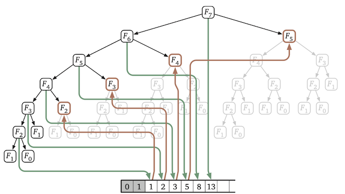
This new recursion tree + memoization array reveals something new about how our algorithm is behaving. Every entry in the array is written to before it is used (as one would hope), and the writing is done entry by entry from left to right/least index to largest. We can even imagine there are two more entries for F[0] and F[1] (depicted above in gray boxes) that are written to before we start and read from just like any values. It takes O(1) additions to compute each entry, and there are O(n) entries to fill in, so the algorithm must use O(n) additions total.²

That process almost sounds iterative. So why don’t we but out the middle-Fairy and make the iteration explicit?

Now the algorithm very clearly uses O(n) additions total.

Dynamic programming

We’ve just seen our first example of dynamic programming, popularized by Richard Bellman in the mid 1950s even though others like Virahanka and Fibonacci had been using similar ideas for centuries already.

It’s not just about applying memoization to a recursive algorithm. And it’s especially not about ignoring recursion and jumping straight to filling in tables. (Seriously, that mindset leads to incorrect algorithms, frustrated graders, and 0s on your graded work.)

Dynamic programming a whole process described in the textbook and on the second page of Lab 7b and in the default dynamic programming grading rubric. Also, there’s a reminder in scary red text about the rubric on the top of Homework 6.

Seriously, please please please read one or preferably all of these descriptions and take them to heart. I recommend the lab handout and the default rubric. I’ll fill in the details as we go through our second example today, but the process has two main stages:

1. Formulate the problem recursively including defining your subproblems carefully so we (and you!) can tell you’re solving them correctly. This is the hard part.
2. Deliberately build subproblem solutions from the bottom up, typically through an iterative algorithm that records results in an array. This should be the easy part, but you will mess it up if you don’t do the first stage first.

Text segmentation, but fast this time

OK, time to cap off all we’ve done this week. For our final problem in the previous lecture, we saw text segmentation: Given an array A[1~..~n] of letters and a subroutine \text{IsWord} that tells you if a string is a “word”, is A the concatenation of words? We solved this problem using a recursive backtracking approach. By what is obviously not at all a coincidence, we did the first stage in the dynamic programming process.

1. Formulate the problem recursively. There are two steps in this stage of the process:

• Give a specification of the specific problem you are solving recursively. The one we ultimately settled on (or I insisted on) was a function \mathit{Splittable} where \mathit{Splittable}(i) = \text{True} if and only if A[i~..~n] is the concatenation of words. It is important to note what call to make to solve your original problem. For text segmentation, it’s \textit{Splittable(1)}.
• Then, figure out and describe the recursive solution. Let \mathit{IsWord}(i, j) be \text{True} if and only if A[i~..~j] is a word. \mathit{Splittable}(i) = \begin{cases} \text{True} & \text{if $i > n$} \\ \bigvee_{j = i}^n \left(\mathit{IsWord}(i, j) \wedge \mathit{Splittable}(j + 1)\right) & \text{otherwise} \end{cases} Like with Fibonacci numbers, the recurrence itself suggests a recursive algorithm for evaluating it, but running this algorithm directly would be too slow, so now it’s time for the second stage of the process.

2. Build solutions to your recurrence from the bottom up. This stage has several steps. Fortunately, they’re all completely mechanical and should become second nature given “sufficient practice”. Finding a recursive solution is the hard but necessary part. Speeding it up should be (or become) the easy part.

• To create a sufficient data structure for memoization, we need to identify the subproblems. For Fibonacci numbers, it was the integers 0 through n. For text segmentation, the initial call uses 1, and the others use all the greater integers i up to the base case of i = n + 1.

• After identifying subproblems, we may choose our memoization data structure. Usually, it’s a (multidimensional) array. Make sure the indices you declare cover all the subproblem parameters. For Fibonacci numbers, we used an array F[0~..~n]. In text segmentation, we’ll go with \mathit{SplitTable}[1~..~n+1]. DO NOT CALL IT DP. You should give it a meaningful name that helps you remember what it’s for. Just like you do anytime you write code for anything, right?

• Next, we need to figure out how we’re going to fill the data structure. To that end, we need to understand the dependencies each subproblem has on other subproblems’ results. I highly recommend drawing a picture of your memoization data structure, picking a generic element (not a base case), and drawing arrows from each other element it depends upon. For Fibonacci numbers, the dependencies were the two elements to the left (in a horizontal drawing of the array). In text segmentation, it’s all of the elements to the right.

  TODO: Add an example figure for dependencies and evaluation order.

• Now we’re ready to find a good evaluation order. Order the subproblems so they come after those they depend upon. I like to draw a big fat arrow in another color on the same diagram to show it. If you have a multidimensional array, make sure to show which loops enclose other loops. For Fibonacci numbers, we evaluated from left to right. In text segmentation, we need to go from right to left!

• And now you’re ready to write down your algorithm (in practice I mean; see the rubrics). Just copy your recurrence verbatim (or as close as you can) into whatever scaffolding you need to support your evaluation order. If your data structure is an array, it’s probably some nested for loops. Be sure to iterate in the correct direction! Jeff (who wrote the Algorithms book) likes to record the base case(s) separate from the main loops (and doing so when there are a lot of base cases sometimes requires thinner loops). That’s the correct strategy in practice, but I prefer to do all of the case analysis including deciding if we’re in a base case inside the main loops, at least as a first pass when all I care about is that there is an efficient algorithm. Don’t forget to return the value you were actually asked to compute!

  \text{FastSplittable}(A[1~..~n]):

  • for i \gets \text{$n + 1$ down to $1$}
    • if i = n + 1
      • \mathit{SplitTable}[i] \gets \text{True}
    • else
      • \mathit{SplitTable}[i] \gets \text{False}
      • for j \gets \text{$i$ to $n$}
        • if \mathit{IsWord}(i, j) and \mathit{SplitTable}[j + 1]
          • \mathit{SplitTable}[i] \gets \text{True}
  • return \mathit{SplitTable}[1]

• And now that we have our iterative algorithm, it should be very easy to figure out the running time. Because we know nothing about the internal workings or running time of \mathit{IsWord} itself, the most appropriate thing to do here is count how may times we call it: O(n^2).

We could have analyzed running time as early as identifying the subproblems, because all it comes down to is adding up all the running times of the possible subproblems (ignoring the recursive calls). That sum doesn’t depend on the evaluation order or the exact pseudocode you write. Instead, the sum is (often) just # subproblems * time per subproblem. In this case, we have O(n) subproblems but we need O(n) calls to \mathit{IsWord} per subproblem to evaluate the giant OR in the recurrence. Sure enough, O(n) \cdot O(n) = O(n^2). The reason you may want to do the analysis before picking a data structure and evaluation order is so you can determine whether your recursive strategy will lead to an acceptable running time before grinding through the rest of the process.

The lab before this lecture has you design some backtracking algorithms for what we expect to be 3 out of 5 problems over a sequence. The next lab, has you finish the dynamic programming process for all 5 problems. It goes along with what was written above: making correct backtracking algorithms is the hard part, and speeding them up is the easy part. But if you don’t do the hard part first, what should be the easy part will actually end up being the wrong part.

There are two whole lecture remaining on dynamic programming. We’ll look at different patterns you may encounter when designing backtracking algorithms in the first half of the process.

TODO: SubsetSum