Principal Component Analysis
Learning Objectives
- Understand why Principal Component Analysis is an important tool in analyzing data sets
- Know the pros and cons of PCA
- Be able to implement PCA algorithm
What is PCA?
PCA, or Principal Component Analysis, is an algorithm to reduce a large data set without loss of important imformation. PCA is defined as an orthogonal linear transformation that transforms the data to a new coordinate system such that the greatest variance by some scalar projection of the data comes to lie on the first coordinate (called the first principal component), the second greatest variance on the second coordinate, and so on.
In simpler words, it detects the directions for maximum variance and project the original data set to a lower dimensional subspace (up to a change of basis) that still contains most of the important imformation.
- Pros: Only the “least important” variables are omitted, the more valuable variables are kept. Moreover, the created new variables are mutually independent, which is essential for linear models.
- Cons: The new variables created will have different meanings than the original dataset. (Loss of interpretability)
Example
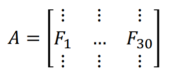
Consider a large dataset with \(m\) samples and 30 different cell features. There are many variables that are highly correlated with each other. We can create an \(m \times\)30 matrix \(\bf A\), with the columns \(\bf F_i\) representing the different features.
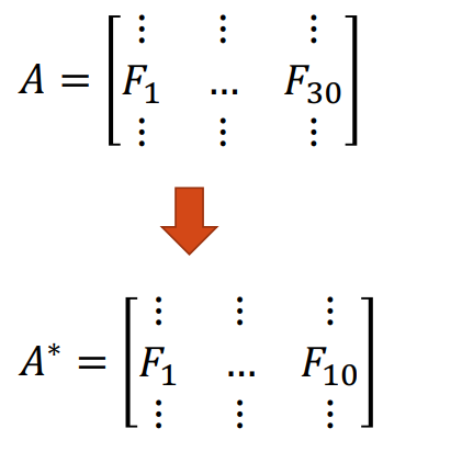
Now suppose we want to reduce the feature space. One method is to directly remove some feature variables. For example, we could ignore the last 20 feature columns to obtain a reduced data matrix \(\bf A^*\). This approach is simple and maintains the interpretation of the feature variables, but we have lost the dropped column information.
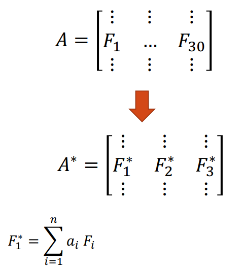
Another approach is to use PCA. We create “new feature variables” \(\bf F_i^*\) from a specific linear combination of the original variables. Each of the new variables after PCA are all independent of one another. Now, we are able to use less variables, but still contain information of all features. The disadvantage here is that we have lost “meaningful” interpretation of the new feature variables.
Data Centering
The first step of PCA is to center the data. We carry out a data shift to our data columns of \(\bf A\) such that each column has a mean of 0. For each feature column \(\bf F_i\) of \(\bf A\), we calculate the mean \(\bar{F_i}\) and do a subtraction of \(\bar{F_i}\) from each entry of the column \(\bf F_i\). We do this procedure to each column, until we obtain a new centered data set \(\bf A\).
Example
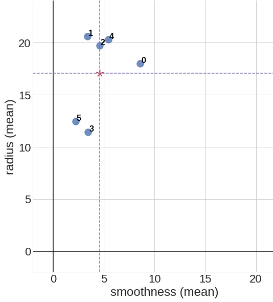
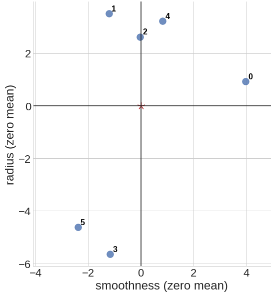
This is an example of data centering for a set of 6 data points \(p_0 = (8.6, 18.0)\), \(p_1 = (3.4, 20.6)\), \(p_2 = (4.6, 19.7)\), \(p_3 = (3.4, 11.4)\), \(p_4 = (5.4, 20.3)\), \(p_5 = (2.2, 12.4)\) on a 2d coordinate space. We first calculate the mean point \(\bar{p} = (4.6, 17.1)\), then shift all of the data points such that our new mean point is centered at \(\bar{p}' = (0, 0)\).
Covariance Matrix
For our centered data set \(\bf A\) of dimension \(m \times n\), where \(m\) is the total number of data points and \(n\) is the number of features, the Covariance Matrix is defined to be
\[Cov({\bf A}) = \frac{1}{m-1} {\bf A}^T {\bf A}.\]The diagonal entries of \(Cov({\bf A})\) explain how each feature correlates with itself, and the sum of the diagonal entries is called the overall variability (total variance) of the problem.
Example
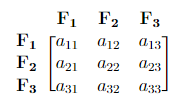
Consider a covariance matrix in the form below. From this matrix, we can obtain:
- \(a_{ii}\) = the variance of each \(\bf F_i\) (How \(\bf F_i\) correlates with itself). Here \(i = 1, 2, 3\).
- \(a_{11} + a_{22} + a_{33}\) = Overall variability (total variance).
- \(\frac{a_{ii}}{a_{11} + a_{22} + a_{33}} \cdot\) 100% = Percentage of the total variance that is explained by \(\bf F_i\). Here \(i = 1, 2, 3\).
Diagonalization and Principal Components
PCA replaces the original feature variables with new variables, called principal components, which are orthogonal (i.e. they have zero covariations) and have variances in decreasing order. To accomplish this, we will use the diagonalization of the covariance matrix.
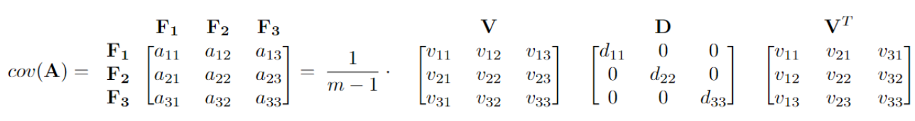
\[Cov({\bf A}) = \frac{1}{m-1} {\bf A}^T {\bf A} = \frac{1}{m-1} {\bf V D} {\bf V}^T.\]Here the columns of \({\bf V}\) are the eigenvectors of \({\bf A}^T {\bf A}\), with the corresponding eigenvalues as the diagonal entries of the diagonal matrix \({\bf D}\). The largest eigenvalue of the covariance matrix corresponds to the largest variance of the dataset, and the associated eigenvector is the direction of maximum variance, called the first principal component.
Example
For the same covariance matrix in the above example, we can write it in the diagonalization form. Here, \(\frac{1}{m-1} \cdot (d_{11} + d_{22} + d_{33})\) sums up to \(a_{11} + a_{22} + a_{33}\), which represents the overall variability. The first column of \({\bf V}\) is the first principal component, and it represents the direction of the maximum variance \(\frac{1}{m-1} \cdot d_{11}\). Here, the first principal component accounts for \(\frac{d_{11}}{d_{11} + d_{22} + d_{33}} \cdot\) 100% of the variability of the question.
SVD and Data Transforming
We know that the eigenvectors of \({\bf A}^T {\bf A}\) are the right singular vectors of \({\bf A}\), or the columns of \({\bf V}\) from the SVD decomposition of \({\bf A}\) (or the rows of V transpose). Hence, instead of having to calculate the covariance matrix and solve an eigenvalue problem, we will instead get the reduced form of the SVD!
From
\[{\bf A} = {\bf U \Sigma V}^T,\]we can obtain the maximum variance as the largest squared singular value of \({\bf A}\), i.e. \({\sigma ^2 _{max}}\), the maximum squared entry of \({\bf \Sigma}\), and the first principal component (direction of maximum variance) as the corresponding column of \({\bf V}\).
Finally, we can transform our dataset with respect to the directions of our principal components:
\[{\bf A}^* := {\bf A V = U \Sigma}.\]\({\bf A V}\) is the projection of the data onto the principal components. \({\bf A V_k}\) is the projection onto the first k principal components, where \({\bf V_k}\) represents the first \(k\) columns of V.
Summary of PCA Algorithm
Suppose we are given a large data set \(\bf A\) of dimension \(m \times n\), and we want to reduce the data set to a smaller one \({\bf A}^*\) of dimension \(m \times k\) without loss of important information. We can achieve this by carrying out PCA algorithm with the following steps:
- Shift the data set \(\bf A\) so that it has zero mean: \({\bf A} = {\bf A} - {\bf A}.mean()\).
- Compute SVD for the original data set: \({\bf A}= {\bf U \Sigma V}^T\).
- Note that the variance of the data set are determined by the singular values of \(\bf A\), i.e. \(\sigma_1, ... , \sigma_n\).
- Note that the columns of \(\bf V\) represent the principal directions of the data set.
- Our new data set is \({\bf A}^* := {\bf AV} ={\bf U\Sigma}\).
- Sometimes we want to reduce the dimension of the data set, and we only use the most important \(k\) principal directions, i.e. the first \(k\) columns of V. Thus we can change the above Equation \({\bf A}^* = {\bf AV}\) to \({\bf A}^* = {\bf AV_k}\), \({\bf A}^*\) has the desired dimension \(m \times k\).
Note that the variance of the data set corresponds to the singular values: \(({\bf A}^*)^T {\bf A}^*= {\bf V}^T{\bf A}^T{\bf AV}={\bf \Sigma}^T{\bf \Sigma}\), as indicated in step 3.
Alternative Definitions of Principal Components
There are other closely related quantities that also have the name principal components. We refer to the principal components as the direction of variances, i.e. the columns of \(\bf V\). In some other cases, the principal components refer to the variances themselves, i.e. \(\sigma_1^2, ... , \sigma_n^2\). In such a case, the direction of variances may be called the principal directions. The meaning of principal components should be clear by the context.
ChangeLog
- 2022-04-18 Yuxuan Chen yuxuan19@illinois.edu: Added PCA definition, data centering, covariance matrix, diagonalization, svd, examples, summary, alternative def
- 2020-08-09 Yikai Teng yikait2@illinois.edu: outline
- 2020-11-30 Jerry Yang jiayiy7@illinois.edu: fix pca code