Singular Value Decompositions

---

Learning Objectives

• Construct an SVD of a matrix
• Identify pieces of an SVD
• Use an SVD to solve a problem

Singular Value Decomposition

An $m\times n$ real matrix $\mathbf{A}$ has a singular value decomposition of the form

$$\mathbf{A}=\mathbf{U}\mathbf{\Sigma }{\mathbf{V}}^T$$

where $\mathbf{U}$ is an $m\times m$ orthogonal matrix, $\mathbf{V}$ is an $n\times n$ orthogonal matrix, and $\mathbf{\Sigma }$ is an $m\times n$ diagonal matrix. Specifically,

• $\mathbf{U}$ is an $m\times m$ orthogonal matrix whose columns are eigenvectors of $\mathbf{A}{\mathbf{A}}^T$. The columns of $\mathbf{U}$ are called the left singular vectors of $\mathbf{A}$.

$$\mathbf{A}{\mathbf{A}}^T=(\mathbf{U}\mathbf{\Sigma }{\mathbf{V}}^T)(\mathbf{U}\mathbf{\Sigma }{\mathbf{V}}^T{)}^T$$ $$=(\mathbf{U}\mathbf{\Sigma }{\mathbf{V}}^T)(({\mathbf{V}}^T{)}^T{\mathbf{\Sigma }}^T{\mathbf{U}}^T)$$ $$=\mathbf{U}\mathbf{\Sigma }({\mathbf{V}}^T\mathbf{V}){\mathbf{\Sigma }}^T{\mathbf{U}}^T$$ $$(\mathbf{V}\text{ is an orthogonal matrix},{\mathbf{V}}^{\mathbf{T}}={\mathbf{V}}^{\mathbf{-}\mathbf{1}}\text{ and }{\mathbf{V}}^T\mathbf{V}=\mathbf{I})$$ $$=\mathbf{U}(\mathbf{\Sigma }{\mathbf{\Sigma }}^T){\mathbf{U}}^T$$

$\mathbf{U}$ is also an orthogonal matrix, we can apply diagonalization ($\mathbf{B}=\mathbf{X}\mathbf{D}{\mathbf{X}}^{\mathbf{-}\mathbf{1}}$).

We have the columns of $\mathbf{U}$ are the eigenvectors of $\mathbf{A}{\mathbf{A}}^T$, with eigenvalues in the diagonal entries of $\mathbf{\Sigma }{\mathbf{\Sigma }}^T$.

• $\mathbf{V}$ is an $n\times n$ orthogonal matrix whose columns are eigenvectors of ${\mathbf{A}}^T\mathbf{A}$. The columns of $\mathbf{V}$ are called the right singular vectors of $\mathbf{A}$.

$${\mathbf{A}}^T\mathbf{A}=(\mathbf{U}\mathbf{\Sigma }{\mathbf{V}}^T{)}^T(\mathbf{U}\mathbf{\Sigma }{\mathbf{V}}^T)$$ $$=\mathbf{V}({\mathbf{\Sigma }}^T\mathbf{\Sigma }){\mathbf{V}}^T$$

Similar to above, we have the columns of $\mathbf{V}$ as the eigenvectors of ${\mathbf{A}}^T\mathbf{A}$, with eigenvalues in the diagonal entries of ${\mathbf{\Sigma }}^T\mathbf{\Sigma }$.

• $\mathbf{\Sigma }$ is an $m\times n$ diagonal matrix of the form:

$$\begin{array}{r}\mathbf{\Sigma }=\left[\begin{array}{ccc}{\sigma }_1& & \\ & \ddots & \\ & & {\sigma }_s\\ 0& & 0\\ ⋮& \ddots & ⋮\\ 0& & 0\end{array}\right]\text{when }m>n,\text{and}\mathbf{\Sigma }=\left[\begin{array}{cccccc}{\sigma }_1& & & 0& \dots & 0\\ & \ddots & & & \ddots & \\ & & {\sigma }_s& 0& \dots & 0\end{array}\right]\text{when}m<n.\end{array}$$

where $s=min(m,n)$ and ${\sigma }_1\ge {\sigma }_2\cdots \ge {\sigma }_s\ge 0$ are the square roots of the eigenvalues values of ${\mathbf{A}}^T\mathbf{A}$. The diagonal entries are called the singular values of $\mathbf{A}$.

Note that if ${\mathbf{A}}^T\mathbf{x}\ne 0$, then ${\mathbf{A}}^T\mathbf{A}$ and $\mathbf{A}{\mathbf{A}}^T$ both have the same eigenvalues:

$$\mathbf{A}{\mathbf{A}}^T\mathbf{x}=\lambda \mathbf{x}$$

$$(left-multiply both sides by ${\mathbf{A}}^T$)

$${\mathbf{A}}^T\mathbf{A}{\mathbf{A}}^T\mathbf{x}={\mathbf{A}}^T\lambda \mathbf{x}$$ $${\mathbf{A}}^T\mathbf{A}({\mathbf{A}}^T\mathbf{x})=\lambda ({\mathbf{A}}^T\mathbf{x})$$

Time Complexity

The time-complexity for computing the SVD factorization of an arbitrary $m\times n$ matrix is $\alpha (m^{2}n+n^3)$, where the constant $\alpha$ ranges from 4 to 10 (or more) depending on the algorithm.

In general, we can define the cost as:

$$\mathcal{O}(m^{2}n+n^3)$$

Reduced SVD

The SVD factorization of a non-square matrix $\mathbf{A}$ of size $m\times n$ can be represented in a reduced format:

• For $m\ge n$: $\mathbf{U}$ is $m\times n$, $\mathbf{\Sigma }$ is $n\times n$, and $\mathbf{V}$ is $n\times n$
• For $m\le n$: $\mathbf{U}$ is $m\times m$, $\mathbf{\Sigma }$ is $m\times m$, and $\mathbf{V}$ is $n\times m$ (note if $\mathbf{V}$ is $n\times m$, then ${\mathbf{V}}^T$ is $m\times n$)

The following figure depicts the reduced SVD factorization (in red) against the full SVD factorizations (in gray).

In general, we will represent the reduced SVD as:

$$\mathbf{A}={\mathbf{U}}_R{\mathbf{\Sigma }}_R{\mathbf{V}}_R^T$$

where ${\mathbf{U}}_R$ is a $m\times s$ matrix, ${\mathbf{V}}_R$ is a $n\times s$ matrix, ${\mathbf{\Sigma }}_R$ is a $s\times s$ matrix, and $s=min(m,n)$.

Example: Computing the SVD

We begin with the following non-square matrix, $\mathbf{A}$

and we will compute the reduced form of the SVD (where here $s=3$):

(1) Compute ${\mathbf{A}}^T\mathbf{A}$:

$${\mathbf{A}}^T\mathbf{A}=\left[\begin{array}{ccc}174& 158& 106\\ 158& 197& 134\\ 106& 134& 127\end{array}\right]$$

(2) Compute the eigenvectors and eigenvalues of ${\mathbf{A}}^T\mathbf{A}$:

$$\begin{gathered} {\lambda }_1=437.479,{\lambda }_2=42.6444,{\lambda }_3=17.8766, \\ {\mathit{v}}_1=\left[\begin{array}{c}0.585051\\ 0.652648\\ 0.481418\end{array}\right],{\mathit{v}}_2=\left[\begin{array}{c}-0.710399\\ 0.126068\\ 0.692415\end{array}\right],{\mathit{v}}_3=\left[\begin{array}{c}0.391212\\ -0.747098\\ 0.537398\end{array}\right] \end{gathered}$$

(3) Construct ${\mathbf{V}}_R$ from the eigenvectors of ${\mathbf{A}}^T\mathbf{A}$:

(4) Construct ${\mathbf{\Sigma }}_R$ from the square roots of the eigenvalues of ${\mathbf{A}}^T\mathbf{A}$:

(5) Find $\mathbf{U}$ by solving $\mathbf{U}\mathbf{\Sigma }=\mathbf{A}\mathbf{V}$. For our reduced case, we can find ${\mathbf{U}}_R=\mathbf{A}{\mathbf{V}}_R{\mathbf{\Sigma }}_R^{-1}$. You could also find $\mathbf{U}$ by computing the eigenvectors of ${\mathbf{A}\mathbf{A}}^T$.

$$\mathbf{U}=\stackrel{A}{\overbrace{\left[\begin{array}{ccc}3& 2& 3\\ 8& 8& 2\\ 8& 7& 4\\ 1& 8& 7\\ 6& 4& 7\end{array}\right]}}\stackrel{V}{\overbrace{\left[\begin{array}{ccc}0.585051& -0.710399& 0.391212\\ 0.652648& 0.126068& -0.747098\\ 0.481418& 0.692415& 0.537398\end{array}\right]}}\stackrel{{\mathrm{\Sigma }}^{-1}}{\overbrace{\left[\begin{array}{ccc}0.047810& 0.0& 0.0\\ 0.0& 0.153133& 0.0\\ 0.0& 0.0& 0.236515\end{array}\right]}}$$ $$\mathbf{U}=\left[\begin{array}{ccc}0.215371& 0.030348& 0.305490\\ 0.519432& -0.503779& -0.419173\\ 0.534262& -0.311021& 0.011730\\ 0.438715& 0.787878& -0.431352\\ 0.453759& 0.166729& 0.738082\end{array}\right]$$

We obtain the following singular value decomposition for $\mathbf{A}$:

Recall that we computed the reduced SVD factorization (i.e. $\mathbf{\Sigma }$ is square, $\mathbf{U}$ is non-square) here.

Rank, null space and range of a matrix

Suppose $\mathbf{A}$ is a $m\times n$ matrix where $m>n$ (without loss of generality):

$$\mathbf{A}={\mathbf{U}\mathbf{\Sigma }\mathbf{V}}^T=\left[\begin{array}{ccccc}|& & |& & |\\ |& & |& & |\\ {\mathbf{u}}_1& \cdots & {\mathbf{u}}_n& \cdots & {\mathbf{u}}_m\\ |& & |& & |\\ |& & |& & |\end{array}\right]\left[\begin{array}{ccc}{\sigma }_1& & \\ & \ddots & \\ & & {\sigma }_n\\ & ⋮& \\ -& 0& -\end{array}\right]\left[\begin{array}{ccc}-& {\mathbf{v}}_1^T& -\\ & ⋮& \\ -& {\mathbf{v}}_n^T& -\end{array}\right]$$

We can re-write the above as:

$$\mathbf{A}=\left[\begin{array}{ccc}|& & |\\ |& & |\\ {\mathbf{u}}_1& \cdots & {\mathbf{u}}_n\\ |& & |\\ |& & |\end{array}\right]\left[\begin{array}{ccc}-& {\sigma }_1{\mathbf{v}}_1^T& -\\ & ⋮& \\ -& {\sigma }_n{\mathbf{v}}_n^T& -\end{array}\right]$$

Furthermore, the product of two matrices can be written as a sum of outer products:

$$\mathbf{A}={\sigma }_1{\mathbf{u}}_1{\mathbf{v}}_1^T+{\sigma }_2{\mathbf{u}}_2{\mathbf{v}}_2^T+...+{\sigma }_n{\mathbf{u}}_n{\mathbf{v}}_n^T$$

For a general rectangular matrix, we have:

$$\mathbf{A}=\sum _{i=1}^s{\sigma }_i{\mathbf{u}}_i{\mathbf{v}}_i^T$$

where $s=min(m,n)$.

If $\mathbf{A}$ has $s$ non-zero singular values, the matrix is full rank, i.e. $\text{rank}(\mathbf{A})=s$.

If $\mathbf{A}$ has $r$ non-zero singular values, and $r<s$, the matrix is rank deficient, i.e. $\text{rank}(\mathbf{A})=r$.

In other words, the rank of $\mathbf{A}$ equals the number of non-zero singular values which is the same as the number of non-zero diagonal elements in $\mathbf{\Sigma }$.

Rounding errors may lead to small but non-zero singular values in a rank deficient matrix. Singular values that are smaller than a given tolerance are assumed to be numerically equivalent to zero, defining what is sometimes called the effective rank.

The right-singular vectors (columns of $\mathbf{V}$) corresponding to vanishing singular values of $\mathbf{A}$ span the null space of $\mathbf{A}$, i.e. null($\mathbf{A}$) = span{${\mathbf{v}}_{r+1}$, ${\mathbf{v}}_{r+2}$, …, ${\mathbf{v}}_n$}.

The left-singular vectors (columns of $\mathbf{U}$) corresponding to the non-zero singular values of $\mathbf{A}$ span the range of $\mathbf{A}$, i.e. range($\mathbf{A}$) = span{${\mathbf{u}}_1$, ${\mathbf{u}}_2$, …, ${\mathbf{u}}_r$}.

Example:

$$\mathbf{A}=\left[\begin{array}{cccc}\frac{1}{\sqrt{2}}& -\frac{1}{\sqrt{2}}& 0& 0\\ \frac{1}{\sqrt{2}}2& \frac{1}{\sqrt{2}}& 0& 0\\ 0& 0& 0& 1\\ 0& 0& 1& 0\end{array}\right]\left[\begin{array}{ccc}14& 0& 0\\ 0& 14& 0\\ 0& 0& 0\\ 0& 0& 0\end{array}\right]\left[\begin{array}{ccc}1& 0& 0\\ 0& 1& 0\\ 0& 0& 1\end{array}\right]$$

The rank of $\mathbf{A}$ is 2.

The vectors $\left[\begin{array}{c}\frac{1}{\sqrt{2}}\\ \frac{1}{\sqrt{2}}\\ 0\\ 0\end{array}\right]$ and $\left[\begin{array}{c}-\frac{1}{\sqrt{2}}\\ \frac{1}{\sqrt{2}}\\ 0\\ 0\end{array}\right]$ provide an orthonormal basis for the range of $\mathbf{A}$.

The vector $\left[\begin{array}{c}0\\ 0\\ 1\end{array}\right]$ provides an orthonormal basis for the null space of $\mathbf{A}$.

(Moore-Penrose) Pseudoinverse

If the matrix $\mathbf{\Sigma }$ is rank deficient, we cannot get its inverse. We define instead the pseudoinverse:

$$({\mathbf{\Sigma }}^{+}{)}_{ii}=\{\begin{array}{ll}\frac{1}{{\sigma }_i}& {\sigma }_i\ne 0\\ 0& {\sigma }_i=0\end{array}$$

For a general non-square matrix $\mathbf{A}$ with known SVD ($\mathbf{A}={\mathbf{U}\mathbf{\Sigma }\mathbf{V}}^T$), the pseudoinverse is defined as:

$${\mathbf{A}}^{+}={\mathbf{V}\mathbf{\Sigma }}^{+}{\mathbf{U}}^T$$

For example, if we consider a $m\times n$ full rank matrix where $m>n$:

$${\mathbf{A}}^{+}=\left[\begin{array}{ccc}|& ...& |\\ {\mathbf{v}}_1& ...& {\mathbf{v}}_n\\ |& ...& |\end{array}\right]\left[\begin{array}{cccccc}1/{\sigma }_1& & & 0& \dots & 0\\ & \ddots & & & \ddots & \\ & & 1/{\sigma }_n& 0& \dots & 0\end{array}\right]{\left[\begin{array}{ccccc}|& & |& & |\\ |& & |& & |\\ {\mathbf{u}}_1& \cdots & {\mathbf{u}}_n& \cdots & {\mathbf{u}}_m\\ |& & |& & |\\ |& & |& & |\end{array}\right]}^T$$

Euclidean norm of matrices

The induced 2-norm of a matrix $\mathbf{A}$ can be obtained using the SVD of the matrix :

$$\begin{array}{rl}\Vert \mathbf{A}{\Vert }_2& =\underset{\Vert \mathbf{x}\Vert =1}{max}\Vert \mathbf{A}\mathbf{x}\Vert =\underset{\Vert \mathbf{x}\Vert =1}{max}\Vert {\mathbf{U}\mathbf{\Sigma }\mathbf{V}}^T\mathbf{x}\Vert \\ & =\underset{\Vert \mathbf{x}\Vert =1}{max}\Vert {\mathbf{\Sigma }\mathbf{V}}^T\mathbf{x}\Vert =\underset{\Vert {\mathbf{V}}^T\mathbf{x}\Vert =1}{max}\Vert {\mathbf{\Sigma }\mathbf{V}}^T\mathbf{x}\Vert =\underset{\Vert y\Vert =1}{max}\Vert \mathbf{\Sigma }y\Vert \end{array}$$

And hence,

$$\Vert \mathbf{A}{\Vert }_2={\sigma }_1$$

In the above equations, all the notations for the norm $\Vert .\Vert$ refer to the $p=2$ Euclidean norm, and we used the fact that $\mathbf{U}$ and $\mathbf{V}$ are orthogonal matrices and hence $\Vert \mathbf{U}{\Vert }_2=\Vert \mathbf{V}{\Vert }_2=1$.

Example:

We begin with the following non-square matrix $\mathbf{A}$:

$$\mathbf{A}=\left[\begin{array}{ccc}3& 2& 3\\ 8& 8& 2\\ 8& 7& 4\\ 1& 8& 7\\ 6& 4& 7\end{array}\right].$$

The matrix of singular values, $\mathbf{\Sigma }$, computed from the SVD factorization is:

Consequently the 2-norm of $\mathbf{A}$ is

Euclidean norm of the inverse of matrices

Following the same derivation as above, we can show that for a full rank $n\times n$ matrix we have:

$$\Vert {\mathbf{A}}^{-1}{\Vert }_2=\frac{1}{{\sigma }_n}$$

where ${\sigma }_n$ is the smallest singular value.

For non-square matrices, we can use the definition of the pseudoinverse (regardless of the rank):

$$\Vert {\mathbf{A}}^{+}{\Vert }_2=\frac{1}{{\sigma }_r}$$

where ${\sigma }_r$ is the smallest non-zero singular value. Note that for a full rank square matrix, we have $\Vert {\mathbf{A}}^{+}{\Vert }_2=\Vert {\mathbf{A}}^{-1}{\Vert }_2$. An exception of the definition above is the zero matrix. In this case, $\Vert {\mathbf{A}}^{+}{\Vert }_2=0$

2-Norm Condition Number

The 2-norm condition number of a matrix $\mathbf{A}$ is given by the ratio of its largest singular value to its smallest singular value:

$${\text{cond}}_2(A)=\Vert \mathbf{A}{\Vert }_2\Vert {\mathbf{A}}^{-1}{\Vert }_2={\sigma }_{max}/{\sigma }_{min}.$$

If the matrix $\mathbf{A}$ is rank deficient, i.e. $\text{rank}(\mathbf{A})<min(m,n)$, then ${\text{cond}}_2(\mathbf{A})=\mathrm{\infty }$.

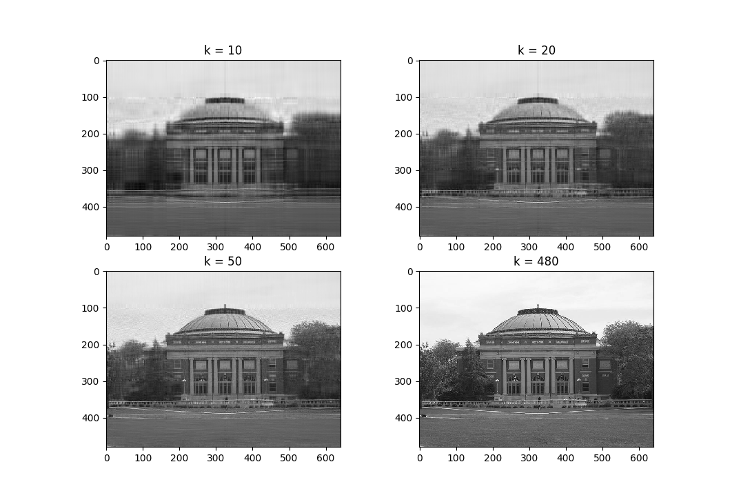
Low-rank Approximation

The best rank-$k$ approximation for a $m\times n$ matrix $\mathbf{A}$, where $k<s=min(m,n)$, for some matrix norm $\Vert .\Vert$, is one that minimizes the following problem:

$$\begin{array}{rl}& \underset{{\mathbf{A}}_k}{min}\Vert \mathbf{A}-{\mathbf{A}}_k\Vert \\ & \text{such that}\mathrm{rank}({\mathbf{A}}_k)\le k.\end{array}$$

Under the induced $2$-norm, the best rank-$k$ approximation is given by the sum of the first $k$ outer products of the left and right singular vectors scaled by the corresponding singular value (where, ${\sigma }_1\ge \cdots \ge {\sigma }_s$):

$${\mathbf{A}}_k={\sigma }_1{\mathbf{u}}_{\mathbf{1}}{\mathbf{v}}_{\mathbf{1}}^{\mathbf{T}}\mathbf{+}\dots {\sigma }_{\mathbf{k}}{\mathbf{u}}_{\mathbf{k}}{\mathbf{v}}_{\mathbf{k}}^{\mathbf{T}}$$

Observe that the norm of the difference between the best approximation and the matrix under the induced $2$-norm condition is the magnitude of the $(k+1{)}^{\text{th}}$ singular value of the matrix:

$$\Vert \mathbf{A}-{\mathbf{A}}_k{\Vert }_2={\left|\left|\sum _{i=k+1}^n{\sigma }_i{\mathbf{u}}_{\mathbf{i}}{\mathbf{v}}_{\mathbf{i}}^{\mathbf{T}}\right|\right|}_2={\sigma }_{k+1}$$

Note that the best rank-$k$ approximation to $\mathbf{A}$ can be stored efficiently by only storing the $k$ singular values ${\sigma }_1,\dots ,{\sigma }_k$, the $k$ left singular vectors ${\mathbf{u}}_{\mathbf{1}}\mathbf{,}\dots \mathbf{,}{\mathbf{u}}_{\mathbf{k}}$, and the $k$ right singular vectors ${\mathbf{v}}_{\mathbf{1}}\mathbf{,}\dots \mathbf{,}{\mathbf{v}}_{\mathbf{k}}$.

The figure below show best rank-$k$ approximations of an image (you can find the code snippet that generates these images in the IPython notebook):

SVD Summary

• The SVD is a factorization of an $m\times n$ matrix $\mathbf{A}$ into $\mathbf{A}=\mathbf{U}\mathbf{\Sigma }{\mathbf{V}}^T$ where $\mathbf{U}$ is an $m\times m$ orthogonal matrix, $\mathbf{V}$ is an $n\times n$ orthogonal matrix, and $\mathbf{\Sigma }$ is an $m\times n$ diagonal matrix.
• Reduced form: $\mathbf{A}={\mathbf{U}}_{\mathbf{R}}{\mathbf{\Sigma }}_{\mathbf{R}}{{\mathbf{V}}_{\mathbf{R}}}^T$ where ${\mathbf{U}}_{\mathbf{R}}$ is an $m\times s$ matrix, ${\mathbf{V}}_{\mathbf{R}}$ is an $n\times s$ matrix, and ${\mathbf{\Sigma }}_{\mathbf{R}}$ is an $s\times s$ diagonal matrix. Here, $s=min(m,n)$.
• The columns of $\mathbf{U}$ are the eigenvectors of the matrix $\mathbf{A}{\mathbf{A}}^T$, and are called the left singular vectors of $\mathbf{A}$.
• The columns of $\mathbf{V}$ are the eigenvectors of the matrix ${\mathbf{A}}^T\mathbf{A}$, and are called the right singular vectors of $\mathbf{A}$.
• The square roots of the eigenvalues of ${\mathbf{A}}^T\mathbf{A}$ are the diagonal entries of $\mathbf{\Sigma }$, called the singular values ${\sigma }_i=\sqrt{{\lambda }_i}$.
• The singular values ${\sigma }_i$ are always non-negative.

Review Questions

• See this review link

ChangeLog

• 2022-04-10 Yuxuan Chen yuxuan19@illinois.edu: added svd proof, changed svd cost, included svd summary
• 2020-04-26 Mariana Silva mfsilva@illinois.edu: adding more details to sections
• 2018-11-14 Erin Carrier ecarrie2@illinois.edu: spelling fix
• 2018-10-18 Erin Carrier ecarrie2@illinois.edu: correct svd cost
• 2018-01-14 Erin Carrier ecarrie2@illinois.edu: removes demo links
• 2017-12-04 Arun Lakshmanan lakshma2@illinois.edu: fix best rank approx, svd image
• 2017-11-15 Erin Carrier ecarrie2@illinois.edu: adds review questions, adds cond num sec, removes normal equations, minor corrections and clarifications
• 2017-11-13 Arun Lakshmanan lakshma2@illinois.edu: first complete draft
• 2017-10-17 Luke Olson lukeo@illinois.edu: outline