Singular Value Decompositions

---

Learning Objectives

• Construct an SVD of a matrix
• Identify pieces of an SVD
• Use an SVD to solve a problem

Singular Value Decomposition

An \(m \times n\) real matrix \({\bf A}\) has a singular value decomposition of the form

$${\bf A} = {\bf U} {\bf \Sigma} {\bf V}^T$$

where

• \({\bf U}\) is an \(m \times m\) orthogonal matrix whose columns are eigenvectors of \({\bf A} {\bf A}^T\). The columns of \({\bf U}\) are called the left singular vectors of \({\bf A}\).
• \({\bf \Sigma}\) is an \(m \times n\) diagonal matrix of the form:

$$\begin{eqnarray} {\bf \Sigma} = \begin{bmatrix} \sigma_1 & & \\ & \ddots & \\ & & \sigma_s \\ 0 & & 0 \\ \vdots & \ddots & \vdots \\ 0 & & 0 \end{bmatrix} \text{when } m > n, \; \text{and} \; {\bf \Sigma} = \begin{bmatrix} \sigma_1 & & & 0 & \dots & 0 \\ & \ddots & & & \ddots &\\ & & \sigma_s & 0 & \dots & 0 \\ \end{bmatrix} \text{when} \, m < n. \end{eqnarray}$$

where $s = \min(m,n)$ and \(\sigma_1 \ge \sigma_2 \dots \ge \sigma_s \ge 0\) are the square roots of the eigenvalues values of \({\bf A}^T {\bf A}\). The diagonal entries are called the singular values of \({\bf A}\).

Note that if $\mathbf{A}^T\mathbf{x} \ne 0$, then $\mathbf{A}^T\mathbf{A}$ and $\mathbf{A}\mathbf{A}^T$ both have the same eigenvalues:

$$\mathbf{A}\mathbf{A}^T\mathbf{x} = \lambda \mathbf{x}$$

$\hspace{13cm}$(left-multiply both sides by $\mathbf{A}^T$)

$$\mathbf{A}^T\mathbf{A}\mathbf{A}^T\mathbf{x} = \mathbf{A}^T \lambda \mathbf{x}$$ $$\mathbf{A}^T\mathbf{A}(\mathbf{A}^T\mathbf{x}) = \lambda (\mathbf{A}^T\mathbf{x})$$

• \({\bf V}\) is an \(n \times n\) orthogonal matrix whose columns are eigenvectors of \({\bf A}^T {\bf A}\) The columns of \( {\bf V}\) are called the right singular vectors of \({\bf A}\).

Time Complexity

The time-complexity for computing the SVD factorization of an arbitrary \(m \times n\) matrix is proportional to $m^2n + n^3$, where the constant of proportionality ranges from 4 to 10 (or more) depending on the algorithm.

In general, we can define the cost as:

$$\mathcal{O}(m^2n + n^3)$$

Reduced SVD

The SVD factorization of a non-square matrix \({\bf A}\) of size \(m \times n\) can be represented in a reduced format:

• For \(m \ge n\): \({\bf U}\) is \(m \times n\), \({\bf \Sigma}\) is \(n \times n\), and \({\bf V}\) is \(n \times n\)
• For \(m \le n\): \({\bf U}\) is \(m \times m\), \({\bf \Sigma}\) is \(m \times m\), and \({\bf V}\) is \(n \times m\) (note if \({\bf V}\) is \(n \times m\), then \({\bf V}^T\) is \(m \times n\))

The following figure depicts the reduced SVD factorization (in red) against the full SVD factorizations (in gray).

In general, we will represent the reduced SVD as:

$${\bf A} = {\bf U}_R {\bf \Sigma}_R {\bf V}_R^T$$

where ${\bf U}_R$ is a $m \times s$ matrix, ${\bf V}_R$ is a $n \times s$ matrix, ${\bf \Sigma}_R$ is a $s \times s$ matrix, and $s = \min(m,n)$.

Example: Computing the SVD

We begin with the following non-square matrix, \({\bf A}\)

and we will compute the reduced form of the SVD (where here $s = 3$):

(1) Compute \({\bf A}^T {\bf A}\):

$${\bf A}^T {\bf A} = \left[ \begin{array}{ccc} 174 & 158 & 106 \\ 158 & 197 & 134 \\ 106 & 134 & 127 \\ \end{array} \right]$$

(2) Compute the eigenvectors and eigenvalues of \({\bf A}^T {\bf A}\):

$$\lambda_1 = 437.479, \quad \lambda_2 = 42.6444, \quad \lambda_3 = 17.8766, \\ \boldsymbol{v}_1 = \begin{bmatrix} 0.585051 \\ 0.652648 \\ 0.481418\end{bmatrix}, \quad \boldsymbol{v}_2 = \begin{bmatrix} -0.710399 \\ 0.126068 \\ 0.692415 \end{bmatrix}, \quad \boldsymbol{v}_3 = \begin{bmatrix} 0.391212 \\ -0.747098 \\ 0.537398 \end{bmatrix}$$

(3) Construct \({\bf V}_R\) from the eigenvectors of \({\bf A}^T {\bf A}\):

(4) Construct \({\bf \Sigma}_R\) from the square roots of the eigenvalues of \({\bf A}^T {\bf A}\):

(5) Find \({\bf U}\) by solving \({\bf U}{\bf\Sigma} = {\bf A}{\bf V}\). For our reduced case, we can find \({\bf U}_R = {\bf A}{\bf V}_R {\bf \Sigma}_R^{-1}\). You could also find \({\bf U}\) by computing the eigenvectors of \({\bf AA}^T\).

$${\bf U} = \overbrace{\left[ \begin{array}{ccc} 3 & 2 & 3 \\ 8 & 8 & 2 \\ 8 & 7 & 4 \\ 1 & 8 & 7 \\ 6 & 4 & 7 \\ \end{array} \right]}^{A} \overbrace{\left[ \begin{array}{ccc} 0.585051 & -0.710399 & 0.391212 \\ 0.652648 & 0.126068 & -0.747098 \\ 0.481418 & 0.692415 & 0.537398 \\ \end{array} \right]}^{V} \overbrace{\left[ \begin{array}{ccc} 0.047810 & 0.0 & 0.0 \\ 0.0 & 0.153133 & 0.0 \\ 0.0 & 0.0 & 0.236515 \\ \end{array} \right]}^{\Sigma^{-1}}$$ $${\bf U} = \left[ \begin{array}{ccc} 0.215371 & 0.030348 & 0.305490 \\ 0.519432 & -0.503779 & -0.419173 \\ 0.534262 & -0.311021 & 0.011730 \\ 0.438715 & 0.787878 & -0.431352\\ 0.453759 & 0.166729 & 0.738082\\ \end{array} \right]$$

We obtain the following singular value decomposition for \({\bf A}\):

Recall that we computed the reduced SVD factorization (i.e. \({\bf \Sigma}\) is square, \({\bf U}\) is non-square) here.

Rank, null space and range of a matrix

Suppose ${\bf A}$ is a $m \times n$ matrix where $m > n$ (without loss of generality):

$${\bf A}= {\bf U\Sigma V}^{T} = \begin{bmatrix}\vert & & \vert & & \vert \\ \vert & & \vert & & \vert \\ {\bf u}_1 & \cdots & {\bf u}_n & \cdots & {\bf u}_m\\ \vert & & \vert & & \vert \\\vert & & \vert & & \vert \end{bmatrix} \begin{bmatrix} \sigma_1 & & \\ & \ddots & \\ & & \sigma_n \\ & \vdots & \\ -& 0& -\end{bmatrix} \begin{bmatrix} - & {\bf v}_1^T & - \\ & \vdots & \\ - & {\bf v}_n^T & - \end{bmatrix}$$

We can re-write the above as:

$${\bf A} = \begin{bmatrix}\vert & & \vert \\ \vert & & \vert \\ {\bf u}_1 & \cdots & {\bf u}_n \\ \vert & & \vert \\ \vert & & \vert \end{bmatrix} \begin{bmatrix} - & \sigma_1 {\bf v}_1^T & - \\ & \vdots & \\ - & \sigma_n{\bf v}_n^T & - \end{bmatrix}$$

Furthermore, the product of two matrices can be written as a sum of outer products:

$${\bf A} = \sigma_1 {\bf u}_1 {\bf v}_1^T + \sigma_2 {\bf u}_2 {\bf v}_2^T + ... + \sigma_n {\bf u}_n {\bf v}_n^T$$

For a general rectangular matrix, we have:

$${\bf A} = \sum_{i=1}^{s} \sigma_i {\bf u}_i {\bf v}_i^T$$

where $s = \min(m,n)$.

If ${\bf A}$ has $s$ non-zero singular values, the matrix is full rank, i.e. $\text{rank}({\bf A}) = s$.

If ${\bf A}$ has $r$ non-zero singular values, and $r < s$, the matrix is rank deficient, i.e. $\text{rank}({\bf A}) = r$.

In other words, the rank of ${\bf A}$ equals the number of non-zero singular values which is the same as the number of non-zero diagonal elements in ${\bf \Sigma}$.

Rounding errors may lead to small but non-zero singular values in a rank deficient matrix. Singular values that are smaller than a given tolerance are assumed to be numerically equivalent to zero, defining what is sometimes called the effective rank.

The right-singular vectors (columns of ${\bf V}$) corresponding to vanishing singular values of ${\bf A}$ span the null space of ${\bf A}$, i.e. null(${\bf A}$) = span{${\bf v}_{r+1}$, ${\bf v}_{r+2}$, …, ${\bf v}_{n}$}.

The left-singular vectors (columns of ${\bf U}$) corresponding to the non-zero singular values of ${\bf A}$ span the range of ${\bf A}$, i.e. range(${\bf A}$) = span{${\bf u}_{1}$, ${\bf u}_{2}$, …, ${\bf u}_{r}$}.

Example:

$${\bf A} = \left[ \begin{array}{cccc} \frac{1}{\sqrt{2}} & -\frac{1}{\sqrt{2}} & 0 & 0 \\ \frac{1}{\sqrt{2}}2 &\frac{1}{\sqrt{2}} & 0 & 0 \\ 0 & 0 & 0 & 1 \\ 0 & 0 & 1 & 0 \end{array} \right] \left[ \begin{array}{ccc} 14 & 0 & 0 \\ 0 & 14 & 0 \\ 0 & 0 & 0 \\ 0 & 0 & 0 \end{array} \right] \left[ \begin{array}{ccc} 1 & 0 & 0 \\ 0 & 1 & 0 \\ 0 & 0 & 1 \end{array} \right]$$

The rank of ${\bf A}$ is 2.

The vectors $\left[ \begin{array}{c} \frac{1}{\sqrt{2}} \\ \frac{1}{\sqrt{2}} \\ 0 \\ 0 \end{array} \right]$ and $\left[ \begin{array}{c} -\frac{1}{\sqrt{2}} \\ \frac{1}{\sqrt{2}} \\ 0 \\ 0 \end{array} \right]$ provide an orthonormal basis for the range of ${\bf A}$.

The vector $\left[ \begin{array}{c} 0 \\ 0\\ 1 \end{array} \right]$ provides an orthonormal basis for the null space of ${\bf A}$.

(Moore-Penrose) Pseudoinverse

If the matrix ${\bf \Sigma}$ is rank deficient, we cannot get its inverse. We define instead the pseudoinverse:

$$({\bf \Sigma}^+)_{ii} = \begin{cases} \frac{1}{\sigma_i} & \sigma_i \neq 0\\ 0 & \sigma_i = 0 \end{cases}$$

For a general non-square matrix \({\bf A}\) with known SVD (\({\bf A} = {\bf U\Sigma V}^T\)), the pseudoinverse is defined as:

$${\bf A}^{+} = {\bf V\Sigma}^{+}{\bf U}^T$$

For example, if we consider a $m \times n$ full rank matrix where $m > n$:

$${\bf A}^{+}= \begin{bmatrix} \vert & ... & \vert \\ {\bf v}_1 & ... & {\bf v}_n\\ \vert & ... & \vert \end{bmatrix} \begin{bmatrix} 1/\sigma_1 & & & 0 & \dots & 0 \\ & \ddots & & & \ddots &\\ & & 1/\sigma_n & 0 & \dots & 0 \\ \end{bmatrix} \begin{bmatrix}\vert & & \vert & & \vert \\ \vert & & \vert & & \vert \\ {\bf u}_1 & \cdots & {\bf u}_n & \cdots & {\bf u}_m\\ \vert & & \vert & & \vert \\\vert & & \vert & & \vert \end{bmatrix}^T$$

Euclidean norm of matrices

The induced 2-norm of a matrix ${\bf A}$ can be obtained using the SVD of the matrix :

$$\begin{align} \| {\bf A} \|_2 &= \max_{\|\mathbf{x}\|=1} \|\mathbf{A x}\| = \max_{\|\mathbf{x}\|=1} \|\mathbf{U \Sigma V}^T {\bf x}\| \\ & =\max_{\|\mathbf{x}\|=1} \|\mathbf{ \Sigma V}^T {\bf x}\| = \max_{\|\mathbf{V}^T{\bf x}\|=1} \|\mathbf{ \Sigma V}^T {\bf x}\| =\max_{\|y\|=1} \|\mathbf{ \Sigma} y\| \end{align}$$

And hence,

$$\| {\bf A} \|_2= \sigma_1$$

In the above equations, all the notations for the norm $\| . \|$ refer to the $p=2$ Euclidean norm, and we used the fact that ${\bf U}$ and ${\bf V}$ are orthogonal matrices and hence $\|{\bf U}\|_2 = \|{\bf V}\|_2 = 1$.

Example:

We begin with the following non-square matrix ${\bf A}$:

$${\bf A} = \left[ \begin{array}{ccc} 3 & 2 & 3 \\ 8 & 8 & 2 \\ 8 & 7 & 4 \\ 1 & 8 & 7 \\ 6 & 4 & 7 \\ \end{array} \right].$$

The matrix of singular values, \({\bf \Sigma}\), computed from the SVD factorization is:

Consequently the 2-norm of \({\bf A}\) is

Euclidean norm of the inverse of matrices

Following the same derivation as above, we can show that for a full rank $n \times n$ matrix we have:

$$\| {\bf A}^{-1} \|_2= \frac{1}{\sigma_n}$$

where ${\sigma_n}$ is the smallest singular value.

For non-square matrices, we can use the definition of the pseudoinverse (regardless of the rank):

$$\| {\bf A}^{+} \|_2= \frac{1}{\sigma_r}$$

where ${\sigma_r}$ is the smallest non-zero singular value. Note that for a full rank square matrix, we have $\| {\bf A}^{+} \|_2 = \| {\bf A}^{-1} \|_2$. An exception of the definition above is the zero matrix. In this case, $\| {\bf A}^{+} \|_2 = 0$

2-Norm Condition Number

The 2-norm condition number of a matrix \({\bf A}\) is given by the ratio of its largest singular value to its smallest singular value:

$$\text{cond}_2(A) = \|{\bf A}\|_2 \|{\bf A}^{-1}\|_2 = \sigma_{\max}/\sigma_{\min}.$$

If the matrix ${\bf A}$ is rank deficient, i.e. $\text{rank}({\bf A}) < \min(m,n)$, then $\text{cond}_2({\bf A}) = \infty$.

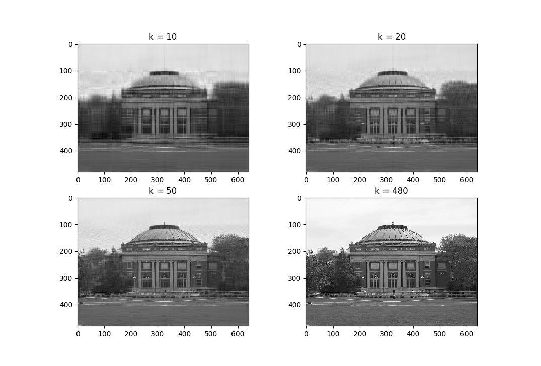
Low-rank Approximation

The best rank-$k$ approximation for a $m \times n$ matrix ${\bf A}$, where $k < s = \min(m,n)$, for some matrix norm $\|.\|$, is one that minimizes the following problem:

$$\begin{aligned} &\min_{ {\bf A}_k } \ \|{\bf A} - {\bf A}_k\| \\ &\textrm{such that} \quad \mathrm{rank}({\bf A}_k) \le k. \end{aligned}$$

Under the induced \(2\)-norm, the best rank-\(k\) approximation is given by the sum of the first \(k\) outer products of the left and right singular vectors scaled by the corresponding singular value (where, \(\sigma_1 \ge \dots \ge \sigma_s\)):

$${\bf A}_k = \sigma_1 \bf{u}_1 \bf{v}_1^T + \dots \sigma_k \bf{u}_k \bf{v}_k^T$$

Observe that the norm of the difference between the best approximation and the matrix under the induced \(2\)-norm condition is the magnitude of the \((k+1)^\text{th}\) singular value of the matrix:

$$\|{\bf A} - {\bf A}_k\|_2 = \left|\left|\sum_{i=k+1}^n \sigma_i \bf{u}_i \bf{v}_i^T\right|\right|_2 = \sigma_{k+1}$$

Note that the best rank-${k}$ approximation to ${\bf A}$ can be stored efficiently by only storing the ${k}$ singular values ${\sigma_1,\dots,\sigma_k}$, the ${k}$ left singular vectors ${\bf u_1,\dots,\bf u_k}$, and the ${k}$ right singular vectors ${\bf v_1,\dots, \bf v_k}$.

The figure below show best rank-\(k\) approximations of an image (you can find the code snippet that generates these images in the IPython notebook):

Review Questions

• See this review link

ChangeLog

• 2020-04-26 Mariana Silva mfsilva@illinois.edu: adding more details to sections
• 2018-11-14 Erin Carrier ecarrie2@illinois.edu: spelling fix
• 2018-10-18 Erin Carrier ecarrie2@illinois.edu: correct svd cost
• 2018-01-14 Erin Carrier ecarrie2@illinois.edu: removes demo links
• 2017-12-04 Arun Lakshmanan lakshma2@illinois.edu: fix best rank approx, svd image
• 2017-11-15 Erin Carrier ecarrie2@illinois.edu: adds review questions, adds cond num sec, removes normal equations, minor corrections and clarifications
• 2017-11-13 Arun Lakshmanan lakshma2@illinois.edu: first complete draft
• 2017-10-17 Luke Olson lukeo@illinois.edu: outline