Graphs and Markov chains

Learning Objectives

Express a graph as a sparse matrix.
Identify the performance benefits of a sparse matrix.

Graphs

Undirected Graphs:

The following is an example of an undirected graph:

The adjacency matrix, ${\bf A}$ , for undirected graphs is always symmetric and is defined as:

$a_{ij} = \begin{cases} 1 \quad \mathrm{if} \ (\mathrm{node}_i, \mathrm{node}_j) \ \textrm{are connected} \\ 0 \quad \mathrm{otherwise} \end{cases},$

where $a_{ij}$ is the $(i,j)$ element of ${\bf A}$ . The adjacency matrix which describes the example graph above is:

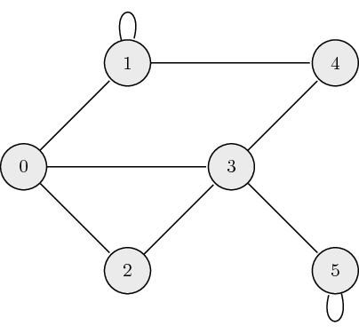
${\bf A} = \begin{bmatrix} 0 & 1 & 1 & 1 & 0 & 0 \\ 1 & 1 & 0 & 0 & 1 & 0 \\ 1 & 0 & 0 & 1 & 0 & 0 \\ 1 & 0 & 1 & 0 & 1 & 1 \\ 0 & 1 & 0 & 1 & 0 & 0 \\ 0 & 0 & 0 & 1 & 0 & 1 \end{bmatrix}.$

Directed Graphs:

The following is an example of a directed graph:

The adjacency matrix, ${\bf A}$ , for directed graphs is defined as:

$a_{ij} = \begin{cases} 1 \quad \mathrm{if} \ \mathrm{node}_i \leftarrow \mathrm{node}_j \\ 0 \quad \mathrm{otherwise} \end{cases},$

where $a_{ij}$ is the $(i,j)$ element of ${\bf A}$ . The adjacency matrix which describes the example graph above is:

${\bf A} = \begin{bmatrix} 0 & 0 & 0 & 1 & 0 & 0 \\ 1 & 1 & 0 & 0 & 0 & 0 \\ 1 & 0 & 0 & 0 & 0 & 0 \\ 0 & 0 & 1 & 0 & 1 & 0 \\ 0 & 1 & 0 & 0 & 0 & 0 \\ 0 & 0 & 0 & 1 & 0 & 1 \end{bmatrix}.$

Weighted Directed Graphs:

The following is an example of a weighted directed graph:

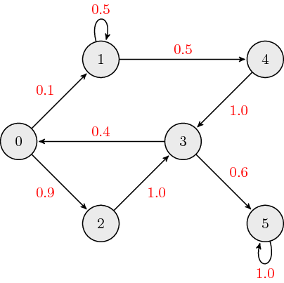
The adjacency matrix, ${\bf A}$ , for weighted directed graphs is defined as:

$a_{ij} = \begin{cases} w_{ij} \quad \mathrm{if} \ \mathrm{node}_i \leftarrow \mathrm{node}_j \\ 0 \quad \ \ \mathrm{otherwise} \end{cases},$

where $a_{ij}$ is the $(i,j)$ element of ${\bf A}$ , and $w_{ij}$ is the link weight associated with edge connecting nodes $i$ and $j$ . The adjacency matrix which describes the example graph above is:

${\bf A} = \begin{bmatrix} 0 & 0 & 0 & 0.4 & 0 & 0 \\ 0.1 & 0.5 & 0 & 0 & 0 & 0 \\ 0.9 & 0 & 0 & 0 & 0 & 0 \\ 0 & 0 & 1.0 & 0 & 1.0 & 0 \\ 0 & 0.5 & 0 & 0 & 0 & 0 \\ 0 & 0 & 0 & 0.6 & 0 & 1.0 \end{bmatrix}.$

Typically, when we discuss weighted directed graphs it is in the context of transition matrices for Markov chains where the link weights across each column sum to $1$ .

Markov Chain

A Markov chain is a stochastic model where the probability of future (next) state depends only on the most recent (current) state. This memoryless property of a stochastic process is called Markov property. From a probability perspective, the Markov property implies that the conditional probability distribution of the future state (conditioned on both past and current states) depends only on the current state.

Markov Matrix

A Markov/Transition/Stochastic matrix is a square matrix used to describe the transitions of a Markov chain. Each of its entries is a non-negative real number representing a probability. Based on Markov property, next state vector ${\bf x}_{k+1}$ is obtained by left-multiplying the Markov matrix with the current state vector ${\bf x}_k$ .

${\bf x}_{k+1} = {\bf M} {\bf x}_k$

In this course, unless specifically stated otherwise, we define the transition matrix ${\bf M}$ as a left Markov matrix where each column sums to $1$ .

Note: Alternative definitions in outside resources may present ${\bf M}$ as a right markov matrix where each row of sums to and the next state is obtained by right-multiplying by , i.e. ${\bf x}_{k+1}^T = {\bf x}_k^T {\bf M}$ .

A steady state vector ${\bf x}^*$ is a probability vector (entries are non-negative and sum to $1$ ) that is unchanged by the operation with the Markov matrix $M$ , i.e.

${\bf M} {\bf x}^* = {\bf x}^*$

Therefore, the steady state vector ${\bf x}^*$ is an eigenvector corresponding to the eigenvalue $\lambda=1$ of matrix . If there is more than one eigenvector with $\lambda=1$ , then a weighted sum of the corresponding steady state vectors will also be a steady state vector. Therefore, the steady state vector of a Markov chain may not be unique and could depend on the initial state vector.

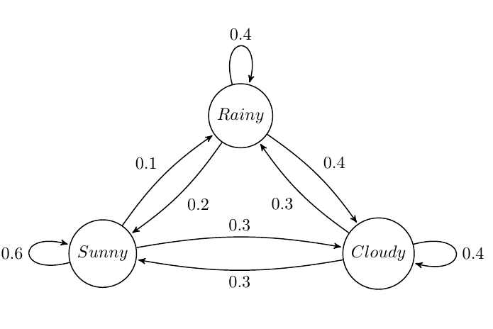
Markov Chain Example

Suppose we want to build a Markov Chain model for weather predicting in UIUC during summer. We observed that:

a sunny day is $60\%$ likely to be followed by another sunny day, $10\%$ likely followed by a rainy day and $30\%$ likely followed by a cloudy day;
a rainy day is $40\%$ likely to be followed by another rainy day, $20\%$ likely followed by a sunny day and $40\%$ likely followed by a cloudy day;
a cloudy day is $40\%$ likely to be followed by another cloudy day, $30\%$ likely followed by a rainy day and $30\%$ likely followed by a sunny day.

The state diagram is shown below:

The Markov matrix is

${\bf M} = \begin{bmatrix} 0.6 & 0.2 & 0.3 \\ 0.1 & 0.4 & 0.3 \\ 0.3 & 0.4 & 0.4 \end{bmatrix}.$

If the weather on day $0$ is known to be rainy, then

${\bf x}_0 = \begin{bmatrix} 0 \\ 1 \\ 0 \end{bmatrix};$

and we can determine the probability vector for day $1$ by

${\bf x}_1 = {\bf M} {\bf x}_0.$

The probability distribution for the weather on day $n$ is given by

${\bf x}_n = {\bf M}^{n} {\bf x}_0.$

Review Questions

See this review link

ChangeLog

2018-04-01 Erin Carrier ecarrie2@illinois.edu: Minor reorg and formatting changes
2018-03-25 Yu Meng yumeng5@illinois.edu: adds Markov chains
2018-03-01 Erin Carrier ecarrie2@illinois.edu: adds more review questions
2018-01-14 Erin Carrier ecarrie2@illinois.edu: removes demo links
2017-11-02 Erin Carrier ecarrie2@illinois.edu: adds changelog, fix COO row index error
2017-10-25 Erin Carrier ecarrie2@illinois.edu: adds review questions, minor fixes and formatting changes
2017-10-25 Arun Lakshmanan lakshma2@illinois.edu: first complete draft
2017-10-16 Luke Olson lukeo@illinois.edu: outline