Graphs and Sparse Matrices
Learning Objectives
- Express a graph as a sparse matrix.
- Identify the performance benefits of a sparse matrix.
Links and Other Content
Nothing here yet.
Graphs
Undirected Graphs: The following is an example of an undirected graph:
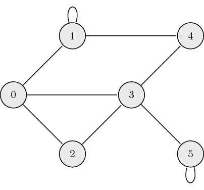
The adjacency matrix, \(A\), for undirected graphs is always symmetric and is defined as: \[ a_{ij} = \begin{cases} 1 \quad \mathrm{if} \ (\mathrm{node}_i, \mathrm{node}_j) \ \textrm{are connected} \\ 0 \quad \mathrm{otherwise} \end{cases}, \] where \(a_{ij}\) is the \((i,j)\) element of \(A\). The adjacency matrix which describes our example graph is: \[ A = \begin{bmatrix} 0 & 1 & 1 & 1 & 0 & 0 \\ 1 & 1 & 0 & 0 & 1 & 0 \\ 1 & 0 & 0 & 1 & 0 & 0 \\ 1 & 0 & 1 & 0 & 1 & 1 \\ 0 & 1 & 0 & 1 & 0 & 0 \\ 0 & 0 & 0 & 1 & 0 & 1 \end{bmatrix}.\]
Directed Graphs: The following is an example of a directed graph:

The adjacency matrix, \(A\), for directed graphs is defined as: \[ a_{ij} = \begin{cases} 1 \quad \mathrm{if} \ \mathrm{node}_i \leftarrow \mathrm{node}_j \\ 0 \quad \mathrm{otherwise} \end{cases}, \] where \(a_{ij}\) is the \((i,j)\) element of \(A\). The adjacency matrix which describes our example graph is: \[ A = \begin{bmatrix} 0 & 0 & 0 & 1 & 0 & 0 \\ 1 & 1 & 0 & 0 & 0 & 0 \\ 1 & 0 & 0 & 0 & 0 & 0 \\ 0 & 0 & 1 & 0 & 1 & 0 \\ 0 & 1 & 0 & 0 & 0 & 0 \\ 0 & 0 & 0 & 1 & 0 & 1 \end{bmatrix}.\]
Weighted Directed Graphs: The following is an example of a weighted directed graph:
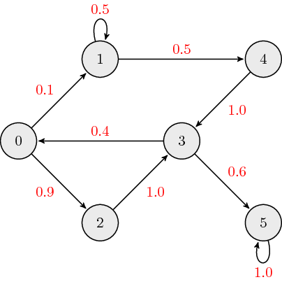
The adjacency matrix, \(A\), for weighted directed graphs is defined as: \[ a_{ij} = \begin{cases} w_{ij} \quad \mathrm{if} \ \mathrm{node}_i \leftarrow \mathrm{node}_j \\ 0 \quad \ \ \mathrm{otherwise} \end{cases}, \] where \(a_{ij}\) is the \((i,j)\) element of \(A\), and \(w_{ij}\) is the link weight associated with edge connecting nodes \(i\) and \(j\). The adjacency matrix which describes our example graph is: \[ A = \begin{bmatrix} 0 & 0 & 0 & 0.4 & 0 & 0 \\ 0.1 & 0.5 & 0 & 0 & 0 & 0 \\ 0.9 & 0 & 0 & 0 & 0 & 0 \\ 0 & 0 & 1.0 & 0 & 1.0 & 0 \\ 0 & 0.5 & 0 & 0 & 0 & 0 \\ 0 & 0 & 0 & 0.6 & 0 & 1.0 \end{bmatrix}.\] Typically, when we discuss weighted directed graphs it is in the context of transition matrices for Markov chains where the link weights across each column sum to \(1\).
Markov Chain
A Markov chain is a stochastic model where the probability of future (next) state depends only on the most recent (current) state. This memoryless property of a stochastic process is called Markov property. From a probability perspective, the Markov property implies that the conditional probability distribution of the future state (conditioned on both past and current states) depends only on the current state.
Markov Matrix
A Markov/Transition/Stochastic matrix is a square matrix used to describe the transitions of a Markov chain. Each of its entries is a non-negative real number representing a probability. Based on Markov property, next state vector \(\boldsymbol{x}_{k+1}\) is obtained by left-multiplying the Markov matrix \(M\) with the current state vector \(\boldsymbol{x}_k\). \[ \boldsymbol{x}_{k+1} = M \boldsymbol{x}_k \] In this course, unless specifically stated otherwise, we define the transition matrix \(M\) as a left Markov matrix where each column sums to \(1\).
Note: Alternative definitions in outside resources may present \(M\) as a right markov matrix where each row of \(M\) sums to \(1\) and the next state is obtained by right-multiplying by \(M\), i.e. \(\boldsymbol{x}_{k+1}^\top = \boldsymbol{x}_k^\top M\).
A steady state vector \(\boldsymbol{x}^*\) is a probability vector (entries are non-negative and sum to \(1\)) that is unchanged by the operation the Markov matrix \(M\), i.e. \[ M \boldsymbol{x}^* = \boldsymbol{x}^* \] Therefore, the steady state vector \(\boldsymbol{x}^*\) is an eigenvector for the eigenvalue \(\lambda=1\) of matrix \(M\). If there is more than one eigenvector with \(\lambda=1\), then a weighted sum of the corresponding steady state vectors will also be a steady state vector. Therefore, the steady state vector of a Markov chain may not be unique and could depend on the initial state vector.
Markov Chain Example
Suppose we want to build a Markov Chain model for weather predicting in UIUC during summer. We observed that:
- a sunny day is \(60\%\) likely to be followed by another sunny day, \(10\%\) likely followed by a rainy day and \(30\%\) likely followed by a cloudy day;
- a rainy day is \(40\%\) likely to be followed by another rainy day, \(20\%\) likely followed by a sunny day and \(40\%\) likely followed by a cloudy day;
- a cloudy day is \(40\%\) likely to be followed by another cloudy day, \(30\%\) likely followed by a rainy day and \(30\%\) likely followed by a sunny day.
The state diagram is shown below:
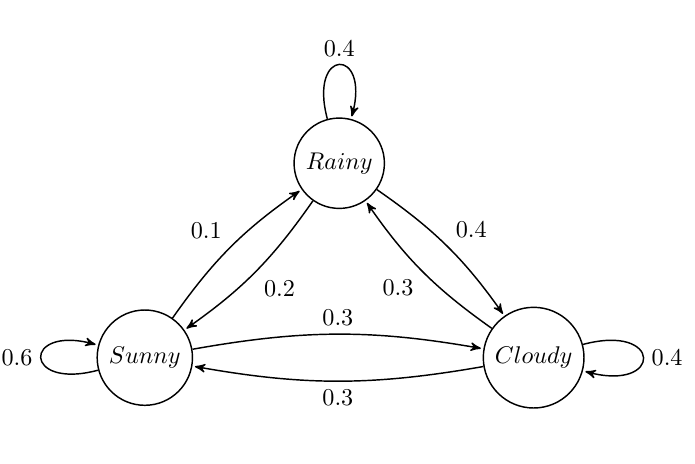
The Markov matrix is \[ M = \begin{bmatrix} 0.6 & 0.2 & 0.3 \\ 0.1 & 0.4 & 0.3 \\ 0.3 & 0.4 & 0.4 \end{bmatrix}. \]
If the weather on day \(0\) is known to be rainy, then \[ \boldsymbol{x}_0 = \begin{bmatrix} 0 \\ 1 \\ 0 \end{bmatrix}; \] and we can determine the probability vector for day \(1\) by \[ \boldsymbol{x}_1 = M \boldsymbol{x}_0. \] The probability distribution for the weather on day \(n\) is given by \[ \boldsymbol{x}_n = M^{n} \boldsymbol{x}_0. \]
Dense Matrices
A \(n \times n\) matrix is called dense if it has \(O(n^2)\) non-zero entries. For example: \[A = \begin{bmatrix} 1.0 & 2.0 & 3.0 \\ 4.0 & 5.0 & 6.0 \\ 7.0 & 8.0 & 9.0 \end{bmatrix}.\]
DNS (Dense Format) stores the matrix dimensions followed by the data values in row major order. For \(A\) the DNS format is: \[AA = \begin{bmatrix} 3 & 3 & 1.0 & 2.0 & 3.0 & 4.0 & 5.0 & 6.0 & 7.0 & 8.0 & 9.0 \end{bmatrix}.\]
Sparse Matrices
A \(n \times n\) matrix is called sparse if it has \(O(n)\) non-zero entries. For example: \[A = \begin{bmatrix} 1.0 & 0 & 0 & 2.0 & 0 \\ 3.0 & 4.0 & 0 & 5.0 & 0 \\ 6.0 & 0 & 7.0 & 8.0 & 9.0 \\ 0 & 0 & 10.0 & 11.0 & 0 \\ 0 & 0 & 0 & 0 & 12.0 \end{bmatrix}.\]
COO (Coordinate Format) stores arrays of row indices, column indices and the corresponding non-zero data values in any order. This format provides fast methods to construct sparse matrices and convert to different sparse formats. For \(A\) the COO format is: \[ \textrm{data} = \begin{bmatrix} 12.0 & 9.0 & 7.0 & 5.0 & 1.0 & 2.0 & 11.0 & 3.0 & 6.0 & 4.0 & 8.0 & 10.0\end{bmatrix}, \\ \textrm{row} = \begin{bmatrix} 4 & 2 & 2 & 1 & 0 & 0 & 3 & 1 & 2 & 1 & 2 & 3 \end{bmatrix}, \\ \textrm{col} = \begin{bmatrix} 4 & 4 & 2 & 3 & 0 & 3 & 3 & 0 & 0 & 1 & 3 & 2 \end{bmatrix}. \]
CSR (Compressed Sparse Row) encodes rows offsets, column indices and the corresponding non-zero data values. This format provides fast arithmetic operations between sparse matrices, and fast matrix vector product. The row offsets are defined by the followign recursive relationship (starting with \(\textrm{rowptr}[0] = 0\)): \[ \textrm{rowptr}[j] = \textrm{rowptr}[j-1] + \mathrm{nnz}(\textrm{row}_{j-1}), \\ \] where \(\mathrm{nnz}(\textrm{row}_k)\) is the number of non-zero elements in the \(k^{th}\) row. Note that the length of \(\textrm{rowptr}\) is \(n_{rows} + 1\), where the last element in \(\textrm{rowptr}\) is the number of nonzeros in \(A\). For \(A\) the CSR format is: \[ \textrm{data} = \begin{bmatrix} 1.0 & 2.0 & 3.0 & 4.0 & 5.0 & 6.0 & 7.0 & 8.0 & 9.0 & 10.0 & 11.0 & 12.0 \end{bmatrix}, \\ \textrm{col} = \begin{bmatrix} 0 & 3 & 0 & 1 & 3 & 0 & 2 & 3 & 4 & 2 & 3 & 4\end{bmatrix}, \\ \textrm{rowptr} = \begin{bmatrix} 0 & 2 & 5 & 9 & 11 & 12 \end{bmatrix}. \]
CSR Matrix Vector Product Algorithm
The following code snippet performs CSR matrix vector product for square matrices:
import numpy as np
def csr_mat_vec(A, x):
  Ax = np.zeros_like(x)
  for i in range(x.shape[0]):
    for k in range(A.rowptr[i], A.rowptr[i+1]):
      Ax[i] += A.data[k]*x[A.col[k]]
  return Ax
Review Questions
- Given an undirected or directed graph (weighted or unweighted), determine the adjacency matrix for the graph.
- What is a transition matrix? Given a graph representing the transitions or a description of the problem, determine the transition matrix.
- For a problem modeled by a Markov matrix, what does a steady-state mean?
- Given an initial state, how can you use a transition matrix to determine the state (probability vector) after 1 timestep? After 2?
- For a Markov chain, what does the state at a given time step depend on?
- What properties must be true for a transition matrix?
- What does it mean for a matrix to be sparse?
- What factors might you consider when deciding how to store a sparse matrix? (Why would you store a matrix in one format over another?)
- Given a sparse matrix, put the matrix in CSR format.
- Given a sparse matrix, put the matrix in COO format.
- For a given matrix, how many bytes total are required to store it in CSR format?
- For a given matrix, how many bytes total are required to store it in COO format?
ChangeLog
- 2018-04-01 Erin Carrier : Minor reorg and formatting changes
- 2018-03-25 Yu Meng : adds Markov chains
- 2018-03-01 Erin Carrier : adds more review questions
- 2018-01-14 Erin Carrier : removes demo links
- 2017-11-02 Erin Carrier : adds changelog, fix COO row index error
- 2017-10-25 Erin Carrier : adds review questions, minor fixes and formatting changes
- 2017-10-25 Arun Lakshmanan : first complete draft
- 2017-10-16 Luke Olson : outline