Learning Objectives

• Practice using binary search trees as dictionaries for large datasets
• Visualize timing differences in competing approaches
• Implement and use a nearest neighbor search (NNS) algorithm
• Solve open-ended code problems with limited provided structure

Getting set up

While most of the mini-project is autograded (and should be submitted like any regular assignment), Prairielearn may not have the physical memory or speed to build a mosaic of your choosing. While it may be possible to do this entire assignment in the provided workspace, you are encouraged to run your code locally as well for improved speed of calculations. If you make your own tileset, you should do so locally.

Assignment Description

A PhotoMosaic is a picture created by taking some source picture, dividing it up into rectangular sections, and replacing each section with a small thumbnail image whose color closely approximates the color of the section it replaces. Viewing the PhotoMosaic at low magnification, the individual pixels appear as the source image, while a closer examination reveals that the image is made up of many smaller tile images.

In this mini-project, you will code up necessary functions to create a mosaic in two different ways (a third solution has already been provided) and observe how the accuracy and speed of three different approaches.

python3 -m pip install --upgrade pip
python3 -m pip install --upgrade Pillow
python3 -m pip install scipy

Python Image Processing

Before we go into the details about your assignment, lets review the format and implementation details of reading in Python Images! Using PNGs (uncompressed image files), we can represent any image as a three-dimensional matrix. For an input image of (width x height) total pixels, this matrix would have the dimensions (width x height x 3) as every pixel in our matrix has three values associated with it. If it helps conceptually, you can also thing of this as 2D array which stores a tuple of size 3 (as we will often use tuples as inputs in this assignment).

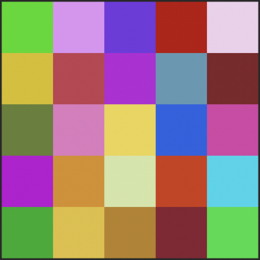
For the following (5 x 5) pixel image, the output numpy array would be:

[[[ 45 218   0], [223 147 243],[116  57 223],[187   9   9], [238 208 236]],
[[216 190  15], [193  64  80], [184  35 215], [ 95 152 180], [128  36  41]],
[[101 128  53], [224 122 191], [237 212  74], [ 35  98 227], [214  66 167]],
[[188   3 211], [217 142  33], [210 229 167], [208  57  22], [  3 213 235]],
[[ 11 172  37], [225 191  57], [184 130  34], [136  33  51], [ 26 220  67]]]

The following functions have been provided for you to assist with reading in and processing images. There are additional helper functions, but you will likely not need to call them (such as squareAndResizeImage() which is called automatically when you loadImage() with a resize value).

#INPUT:
# A string containing the path to a PNG image (fileName)
# An integer containing the square dimension the image should be reduced to (resize)
#OUTPUT:
# A numpy array containing a (row, column, color vector) 3D array
np.array(width x height x color) loadImage(string fileName, int resize = None)

#INPUT:
# rgb_matrix, a numpy array containing a (row, column, color vector) 3D array
#OUTPUT:
# None, instead it writes the image described by rgb_matrix to the file fname
None saveImage(rgb_matrix, fname):

#INPUT:
# A string containing the path to a file location
#OUTPUT:
# A list of strings containing the paths to all valid image files at that location
list[string] listTileImagesInPath(string path)

#INPUT:
# A string containing the path to a file location
# An optional integer argument that will resize the input image into a square of the appropriate size 
#OUTPUT:
# A numpy array storing a 3D (row, col, color) representation of an image
np.array(width x height x color) getTileImage(string fileName, size=None)

Part 1: Naive Mosaic Matching

Given a collection of PNG tiles, we can produce an 100% accurate mosaic at the expense of a very slow runtime by exhaustively comparing every possible tile image for every individual square. In part 1 of this assignment, you must fill in the following functions in order to build a ‘naive’ mosaic constructor.

exactColorDist()

#INPUT:
# c1 and c2, two size-3 tuples as (R, G, B) that are being compared
#OUTPUT:
# A float containing the Euclidian distance between these colors
def exactColorDist(c1, c2):

We can treat three-dimensional colors (RGB-values) as a point in 3D space with values ranging from (0, 0, 0) to (255, 255, 255). You should use the standard Euclidean Distance formula in order to implement this function. Most numbers will not result in ‘clean’ numbers but the autograder has an allowable error tolerance of 0.0001 (if you choose to truncate your calculation for whatever reason).

Input: (255, 0, 0), (255, 255, 0), Output: 255.0
Input: (121, 246, 111), (149, 247, 5), Output: 109.64032105024137

getClosestColor()

#INPUT:
# inList, a list of size-3 tuples containing average colors as (R, G, B)
# query, a size-3 tuple containing the query color of interest
#OUTPUT:
# A size-3 tuple which is the closest match to the input query
# among every item in inlist
# HINT: You will need exactColorDist to solve this.
def getClosestColor(inlist, query):

Write a function that takes in a list of different colors and a single query color (each color is defined as a size-3 tuple) and returns the closest matching color. Here you are intended to use the naive exact approach to loop through every possibility. You are strongly encouraged to use exactColorDist().

There are provided examples in the Python notebook using a ‘rainbow’ dataset to find the closest matching color.

getAverageColor()

#INPUT:
# numArray, a 3D numpy array indexed by [row][col][RGB-color])
# Four optional integer arguments:
# rstart, the starting index (in rows) that must be averaged
# cstart, the starting index (in cols) that must be averaged
# rlen, the number of rows that must be averaged (including the start row)
# clen, the number of cols that must be averaged (including the start col)
# With all four optional arguments, this forms a rectangle. 
# Note the boundaries here: there are only rlen and clen total rows
# (rstart, cstart) to (rstart + rlen - 1, cstart + clen - 1)
# Remember that 0,0 is the top left of an image
#OUTPUT:
# A size-3 tuple containing the average color of the image (or subimage defined by four args)
def getAverageColor(numArray, rstart=0, cstart=0, rlen=None, clen=None):

The default behavior of this function is fairly straightforward. When given a (width x height x color) numpy array, compute the average color of the entire array by taking the average R value, G value, and B value.

NOTE: Remember that RGB values must be integers. In this instance, you should convert whatever float output the average gives to an integer, which will result in truncation math. See the second example below, where the average values are all 127.5, but the appropriate color is 127.

Input: The 5x5x3 matrix given in Figure 1, Output: (153, 125, 114)

Input:                                     Output: (127, 127, 127)
[[[0 0 0][0 0 0]]
[[255 255 255][255 255 255]]]

The complexity of this function comes in when the optional arguments are submitted (you can assume all four optional arguments will always be given if any of them are). When you are given these arguments instead of averaging the entire image (read: the entire numpy array), you should instead average only the rectangular values between points (rstart, cstart) and (rstart+rlen-1, cstart+clen-1). Do you understand why the ‘-1’ is included?

Lets look at the examples below. In the first example, we are starting at position (row=0, col=0) and the total length we are comparing is a 1x1 square. So our average value is just whatever pixel is at (0, 0).

In the second example, we start at (row=1, col=0) and my column length is 2. So I get the average of the first two values in row 1, starting at column 0 [Exact indices: (1, 0), (1, 1)]. They are both (255, 255, 255) so my average is also (255, 255, 255).

In my last example, we start at (row=0, col=0) but our row length is 2. So we get the average of the first value in row 0 and the first value in row 1 [Exact indices: (0, 0), (1, 0)]. This yields an average of (127, 127, 127)

Input: The 5x5x3 matrix given in Figure 1, Output: (45, 218, 0)
rstart=0, cstart=0, rlen=1, clen=1

Input:                                     Output: (255, 255, 255)
[[[0 0 0][0 0 0]]
[[255 255 255][255 255 255]]]
rstart=1, cstart=0, rlen=1, clen=2

Input:                                     Output: (127, 127, 127)
[[[0 0 0][0 0 0]]
[[255 255 255][255 255 255]]]
rstart=0, cstart=0, rlen=2, clen=1

Warning: Successfuly implementing this function (with optional arguments) is key for the mosaic. Otherwise you will not be correctly averaging the color of each square you plan to replace with a new tile image (that most closely matches that square’s average color).

Part 2: Luminance Binary Search Tree

We would like to speed up our nearest neighbor search but without coding up the complexity of a k-d tree. One method of doing this is to convert our multi-dimensional object into a single dimension. Given our objects are RGB color values, there is a meaningful dimension reduction in the form of luminance – a measurement of relative black-white.

The core of this ‘transformation’ is already implemented for you in getLum(), where a simple equation takes in an RGB and returns a single float. Your job is to use this transformation to build a binary search tree capable of finding the nearest neighbor.

lum_tree_insert()

# INPUT: 
# A bstNode containing the root of the tree (or sub-tree) being inserted into. (root)
# A size-3 tuple containing the average color of the image being inserted (key)
# A string containing the path and filename to the image being inserted (val)
# OUTPUT:
# A bstNode containing the root of the tree after the new node has been added
# HINT: Use 'getLum' to compare values as 1D luminance NOT as 3D colors.
bstNode lum_tree_insert(bstNode root, tuple(R, G, B) key, string value):

The luminance tree is a binary search tree where my keys are size-3 tuples containing RGB values (specifically the average value of an image) and my value is a string containing the filename of that image. From an implementation point of view, there is no difference between inserting into a luminance tree and any of the BSTs we have seen in class other than the fact that you must compare 1D luminance values but store size-3 color tuples.

Several small datasets have been provided alongside a build_lum_tree() function for testing the correctness of your insert function. For example:

If I call lum_tree_insert in the following order: [(0, 255, 0), (0, 255, 255), (255, 0, 0), (255, 255, 0), (255, 0, 255), (0, 0, 255)]

The final output is:
        |--(255, 255, 0)
    |--(0, 255, 255)
|--(0, 255, 0)
        |--(255, 0, 255)
    |--(255, 0, 0)
        |--(0, 0, 255)

NOTE: The order of inputs matter and the provided examples in the code may not exactly match with your final output. This is ok – your local machine is not going to store the files in the exact same way and you are likely seeing an issue with the input order moreso than your code. Use the autograder to test for identical trees (as the order will be fixed and run on the same architecture).

lum_tree_find()

# INPUT: 
# A bstNode containing the root of the tree (or sub-tree) being inserted into. (root)
# A size-3 tuple containing the average color being queried (key)
# OUTPUT:
# A bstNode containing the closest match (in luminance) between query and any node in the tree
# HINT: Use 'getLum' to compare values as 1D luminance NOT as 3D colors.
bstNode lum_tree_find(bstNode root, tuple(R, G, B) key):

The nearest neighbor find is very similar to the binary search tree find() function we covered in class. The only difference is that the actual nearest neighbor may be any node along the path we took to the leaf. For example given the tree below, the node (255, 0, 0) does not exactly match our query (90, 75, 50) but it is a closer match than the leaf (255, 0, 255) and the root (0, 255, 0).

Input: 
Given the tree w/ query: (90, 75, 50)
        |--(255, 255, 0)
    |--(0, 255, 255)
|--(0, 255, 0)
        |--(255, 0, 255)
    |--(255, 0, 0)
        |--(0, 0, 255)

Output:
The bstNode with key=(255, 0, 0) and value='data/rainbow/color_0.png'

Part 3: Mosaic Exploration

If you have made it here, congratulations! You now have a Python script capable of reading in large collections of images and producing a mosaic in three different ways. Provided at the bottom of the given notebook are two useful scripts. The first will allow you to convert any PNG into a 80x80 square tile image (the ‘default’ for the instagram dataset provided) while the latter will allow you to create a mosaic from a given image, tileset, and a few additional settings.

Measure the time efficiency of each implementation.

Please measure the time it takes each of the three implementations (naive, luminance, KD-tree) to produce your mosaic while changing a single parameter (the total number of tiles). Then create a line plot with labeled axes and a separate line for each of the implementations with the number of tiles as the x-axis and the time it took to compelte on the y-axis. There should be at least five unique datapoints for each line which are clearly visible in the plot.

Submit a creative mosaic!

While creating your efficiency plot, you are strongly encouraged to try to make your own mosaic(s). As part of this, your final task is to be creative and have fun! Find a target image that you want to convert into a mosaic and find a set of small images you want to use as your replacement tiles. If you cannot find the small tile image, you can also use the instragram imageset (igram). You should not use any of the other test image sets given, as they are monochromatic or random images designed to test your code in human-readable ways (and simply wont produce very interesting ‘mosaics’)

If you are working locally, you may find it helpful to download the instagram mosaic tileset as a zip file HERE.

Your final visualization should be a PNG of an image of your choosing (and ideally using a tileset of your own design). You should run your image with maximumTilesX set to at least 200 and a tileHeight set to at least 16 but can otherwise change your parameters freely. (This includes which implementation you use to produce your final image)