Learning Objectives

• Practice parsing different data formats into graphs
• Create a greedy heuristic algorithm to solve a complex computational problem
• Practice fundamentals of accessing and modifying graphs in NetworkX

Getting set up

This assignment is entirely doable inside Prairielearn.

Assignment Description

For this assignment you are tasked with creating, using, and implementing various graphs and graph algorithms using NetworkX. In part 1, you will create two types of graphs from input data and then produce a simple heuristic for graph coloring. In part 2, you will be given an existing graph structure (a ‘grid’ graph) and need to use NetworkX in order to properly path the nodes visited by an input string pattern. In part 3, you will be given real world data taken from https://openflights.org/data.php and be responsible for converting it into a weighted graph.

Part 1: Graph Coloring

UIUC is drafting up the final exam schedule for the next semester but they’ve decided that the best exam schedule is to simultaneously offer as many exams as possible (and to offer each exam only once). To determine the best schedule in an unbiased way, they plan to use graph coloring – a strategy which assigns a ‘color’ (in this context an exam time slot) to each vertex (in this context a course). By drawing an edge between ever pair of vertices that share at least one student, they can ensure that there are no course conflicts by making sure that the neighbors of every vertex do not share its colors (or in other words, that every course with a student in common doesnt have the same exam time).

This seemingly straightforward problem is actually an NP-complete problem! Given a list of colors for every vertex (a labeling), the correctness of a labeling can be determined very quicky but identifying the smallest number of ‘colors’ that we need to fully label a graph requires a brute-force search in polynomial time (O(n^k)). Instead of brute forcing the exact match solution, we will instead write our own approximate solution as a greedy heuristic. That is to say, we will write an algorithm that is not guaranteed to find the perfect optimal solution, but will get us a valid solution quickly.

Make a complete bipartite graph

# INPUT:
# l1, a list of vertex labels
# l2, a list of vertex labels
# OUTPUT:
# a networkX Graph() where every vertex in l1 has a direct edge
# to every vertex in l2
def make_bipartite_graph(l1, l2):

A bipartite graph is one in which the vertices can be partitioned into two sets where every edge goes between the two sets. In the context of graph coloring, this means that a bipartite graph should always be two-colorable! As a first pass test of our graph coloring algorithm, we will make a complete bipartite graph. This means that every vertex in our first partition should have an edge to every vertex in our second partition.

Consider: Will our graph heuristic be able to color this perfectly?

Random Student Roster Files

# INPUT:
# A line separated csv file storing the course schedule for every student
# The first entry in each row is the student ID followed by a list of classes
# OUTPUT:
# A networkX Graph with course IDs (CSXXX) as nodes and an undirected edge 
# connecting any two classes that share at least one student
def schedule_to_graph(inFile):

The input data format for this mp is a csv file where every student is listed as their own row and a list of courses they are taking is provided. So for example:

Brad, CS101, CS102, CS103
Carl, CS225, CS101

The first line indicates that there is an edge between vertices CS101 and CS102, between CS101 and CS103, and between CS102 and CS103 because Brad is taking all three courses simultaneously (and we need at least three exam slots). The second line shows that there is also an edge between CS225 and CS101 because Carl is taking both courses. Note that this doesnt imply we need four exam slots, because CS225 could be in the CS102 or CS103 exam time! Do you see now how graph coloring is actually quite hard to solve using the minimum amount of colors?

Consider: How do you need to parse this input dataset in order to add all the necessary edges in a NetworkX graph?

The Graph Coloring Heuristic

# INPUT:
# G, a networkX Graph
# node_order, a list of networkX vertex labels in the order they must be colored
# color_list, a list of matplotlib color strings
# OUTPUT:
# None, instead modify every vertex in G to have a new attribute 'color'
# Like the vertex labels, the color order matters:
# The correct color is the first color in the ordered list which is NOT
# used by one or more neighbors.
def colorGraph(G, node_order, color_list):

The graph coloring heuristic we are using is very simple – when at an unlabeled vertex, check all adjacent vertices for colors and pick the first color which does not belong to any neighbor. This approach will not guarantee an optimal (or even very good) coloring scheme but if we enforce a specific order of vertices and possible colors, it will result in a consistent coloring scheme.

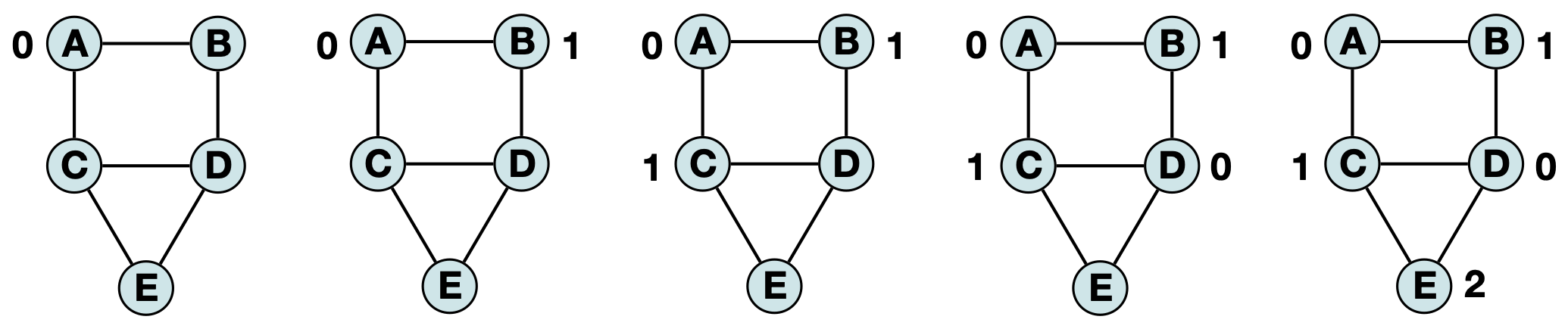
For example, if we ‘visit’ vertices in alphabetical order (A, B, C, D, E) then the heuristic will produce the following labeling (here we will represent colors by numbers for clarity):

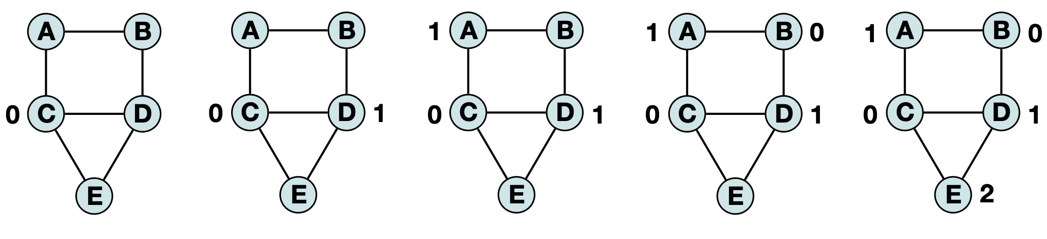
However, if we ‘visit’ vertices in based on the highest degree to lowest degree (C, D, A, B, E) we get a similar (but distinct) labeling:

The provided code base will automatically add a node attribute ‘color’ to every vertex in the input graph but has the default value None. Your job is to modify this graph to have the exact labeling produced by visiting each node and selecting each other in the order provided by the input lists.

To be clear, your function will be graded for an exact reproducibility of the color labeling for a given input but you should be aware that there are usually many valid colorings. In larger and more complex examples, this can result not just a different labeling but a different total number of colors. For the purposes of our motivating problem, we would likely run our heuristic several times on different input node orders to try to approximate the smallest total set of colors is the number of unique exam slots we need to schedule all exams without any course conflicts. As this cannot be reasonably graded, I leave it as an exercise to the reader for those interested in exploring graph algorithms further.

Consider: To get the best possible solution, what is the first vertex we want to visit? What is the last possible vertex we want to visit? If you are interested, try out a few different vertex orderings and see if one consistently outperforms.

Part 2: Pirate Walk

# INPUT:
# inGraph, a networkX Graph() containing a square grid of arbitrary size
# path, a string containing only the characters "N", "S", "E", and "W"
# start, a networkX vertex label that is guaranteed to exist in inGraph
# OUTPUT:
# A list containing the in order visited nodes based on start and path
# The first vertex in the list is always 'start'
def pirate_walk(inGraph, path, start):

Everyone knows that when a pirate is trying to find treasure, they can only walk in the four cardinal directions! You’ve already seen how a pirate could use a list of individual directional steps (“N”, “S”, “E”, “W”) to end up in a totally different position but now its time to extend that knowledge to a full pirate map’s walk – complete with a totally random starting position in a square grid graph!

Given an input graph (which will always be a square grid with correct vertex attributes) and an arbitrary starting position (which will always be a valid vertex label), walk through the graph based on the vertex attribute pos. In other words, your task is to write code capable of looking up all neighbors for your current position and moving in the appropriate direction where:

• North -> y+1
• South -> y-1
• East -> X+1
• West -> X-1

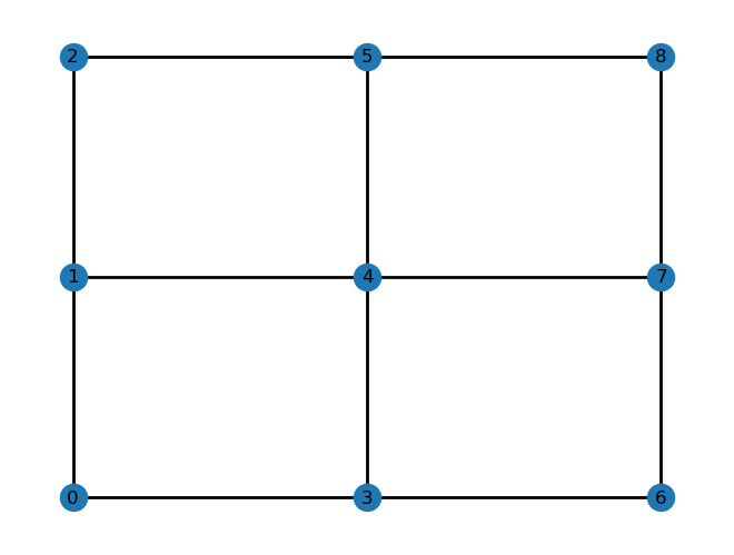
An example square grid with size=3:

An example (with highlighted red path) for size=5, starting node=6 and path=”NNEESW”:

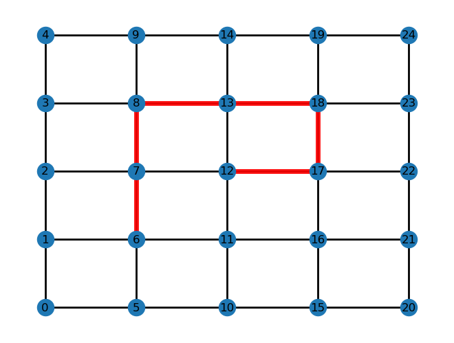
This would have the final return path of [6, 7, 8, 13, 18, 17, 12].

Hint: If you are struggling to figure out where to start, your logic for finding the next vertex in the graph should look at the pos attribute of all neighbors. If you had this information for every neighbor, how would you know which one is the correct neighbor for the next step in the walk?

Part 3: OpenFlights Graph

# INPUT:
# vertex_file, a csv file formatted with the OpenFlights flightpath information for airports
# See the website for details about the format (or https://openflights.org/data.php)
# edge_file, a csv file storing an edge list as an unweighted undirected graph
# OUTPUT:
# A NetworkX weighted graph with airports as nodes with weighted edges between them if there is a flight
# The weight on the edge should match the approximate haversine distance using the provided function
def build_flightpaths_graph(vertex_file, edge_file):

As one final test of your Python data parsing fundamentals applied to a real world dataset, different random subsets of a large airport and flight database have been automatically curated from https://openflights.org/data.php. Your final challenge for this MP is to write code capable of parsing this seemingly messy dataset into a weighted NetworkX graph, where edges each have an attribute ‘weight’ that stores the distance – in kilometers – between any pair of airports with a flight between them.

To assist you in this, a haversine distance function has been provided which will automatically convert longitude and latitute pairs into the appropriate approximate distance. However it is up to you to identify how to read in the CSV file, parse the appropriate columns, and then build the graph from the appropriate edges.

Have fun! Some helpful hints are provided below.

Hint: The openflight website has information about the values in each of the columns in the input vertex file. For your convenience, they are as follows:

1. Airport ID: Unique OpenFlights identifier for this airport.
2. Name of airport: May or may not contain the City name.
3. City Main city served by airport: May be spelled differently from Name.
4. Country: Country or territory where airport is located.
5. IATA: 3-letter IATA code Null if not assigned/unknown.
6. ICAO: 4-letter ICAO code. Null if not assigned.
7. Latitude: Decimal degrees, usually to six significant digits. Negative is South, positive is North.
8. Longitude: Decimal degrees, usually to six significant digits. Negative is West, positive is East.
9. Altitude: In feet.
10. Timezone: Hours offset from UTC. Fractional hours are expressed as decimals, eg. India is 5.5.
11. DST: Daylight savings time.
12. Tz database timezone: Timezone in “tz” (Olson) format, eg. “America/Los_Angeles”.
13. Type: Type of the airport.
14. Source: Source of this data.

Hint: The edge file uses the ICAO 4-letter code with quotes around each code. (‘”’)

This is meant to make your file I/O easier as the ‘raw’ data in the vertex csv file has quotes around all strings. One of your tasks will be to lookup whatever information is necessary to build the weighted edge using the provided csv file about the vertices.