Solo MP This MP, as well as all other MPs in CS 225, are to be completed without a partner.
You are welcome to get help on the MP from course staff, via open lab hours, or Piazza!
Checking Out the Code
All assignments will be distributed via our release repo on github this semester. You will need to have set up your git directory to have our release as a remote repo as described in our git set up
You can merge the assignments as they are released into your personal repo with
git pull --no-edit --no-rebase release main --allow-unrelated-histories
git push
The first git command will fetch and merge changes from the main branch on your remote repository named release into your personal. The --no-edit flag automatically generates a commit message for you, and the--no-rebase flag will merge the upstream branch into the current branch. Generally, these two flags shouldn’t be used, but are included for ease of merging assignments into your repo. Similarly --allow-unrelated-histories will handle issues due to merging the history of our release repo and your own (in which hopefully you are commiting your work).
The second command will push to origin (your personal), which will allow it to track the new changes from release.
You will need to run these commands for every assignment that is released.
All the files for this mp are in the mp_sketching directory.
Preparing Your Code
This semester for MPs we are using CMake rather than just make. This allows for us to use libraries such as Catch2 that can be installed in your system rather than providing them with each assignment. This change does mean that for each assignment you need to use CMake to build your own custom makefiles. To do this you need to run the following in the base directory of the assignment. Which in this assignment is the mp_sketching directory.
mkdir build
cd build
This first makes a new directory in your assignment directory called build. This is where you will actually build the assignment and then moves to that directory. This is not included in the provided code since we are following industry standard practices and you would normally exclude the build directory from any source control system.
Now you need to actually run CMake as follows.
cmake ..
This runs CMake to initialize the current directory which is the build directory you just made as the location to build the assignment. The one argument to CMake here is .. which referes to the parent of the current directory which in this case is top of the assignment. This directory has the files CMake needs to setup your assignment to be build.
At this point you can in the build directory run make as described to build the various programs for the MP.
You will need to do the above once for each assignment. You will need to run make every time you change source code and want to compile it again.
Goals and Overview
In this MP you will:
- Use three different MinHash implementations to create lossy ‘sketches’ of larger datasets
- Use MinHash sketches to approximate similarity between datasets
- Measure the accuracy between exact solutions and approximate solutions
- Create a graph representation of all pairwise minhash estimates
Assignment Description
Sketching algorithms allow us to do very large and computationally intensive data calculations much faster than would otherwise be possible at the cost of some small likelihood of errors (or inaccuracy). In this assignment, you are tasked with writing a code base capable of parsing a large collection of data (either text or PNG). You will then use these functions to create a MinHash sketch representation of moderately sized data collections (test out large on your own!), and then use those sketches to estimate the pairwise similarity of every possible data pair.
To help you accomplish this task, we have split the assignment into testable chunks:
- Part 1 — Creating (and using) MinHash Sketches on integers
- Part 2 — Applying MinHash Sketches to PNGs
- Part 3 — Bulk Analysis of MinHash as a weighted graph
Part 1: Creating MinHash Sketches Three Ways
As seen in lecture, the MinHash sketch is built on the assumption that a good hash function exhibits SUHA-like uniform independence. Under this assumption, by keeping track of some fraction of our overall hash indices (the k-th minimum) we can estimate both the number of unique items in our dataset but also estimate similarity between two datasets by the relative overlap of our minima.
As with most data structures, there are many ways to implement the same underlying idea. For this assignment we will build vectors of minima three different ways. The first approach, k-minima minhash (or kminhash), is the most straightforward and is what most people think of when they hear ‘bottom-k minhash’. Given one hash, we record the k-smallest hash indices from a dataset as a representation of the full dataset. The second, k-hash minhash (or khash_minhash), is the easiest to implement if you have infinite hash functions but is generally considered to be the worst possible implementation (so we will use it in Part 1 and quickly forget about it). Given k unique hashes, we record only the global minimum value for each hash as a representation of the full dataset. We still end up with a set of k minima, but this is only good if we truly have k-independent hash functions. The last, k-partition minhash (or kpartition_minhash), is very useful when our datasets have a high variability in their cardinalities but applying them to cardinality estimation is not something we have seen how to do. (Instead of having the k-th minima, we have k different minima over different ranges.) Much like k-hash, we will use them in Part 1 but generally not consider them in Part 2. To build a k-partition MinHash, we use one hash function but partitions the hashes based on a particular number of its prefix bits. For example, if our hash produces a five-bit index and we use two prefix bits:
Hash Indices (binary): [00110, 01110, 01001, 00111 11100, 11111, 11011]

Bucket 00: [110, 111] # Min Value: 00110
Bucket 01: [110, 001] #Min Value: 01001
Bucket 10: [] # Min Value: 11111 <-- THE GLOBAL MAX INT DENOTES NO MINIMA
Bucket 11: [011, 100, 111] # Min Value 11011
In all three MinHashes, the output of a MinHash sketch is a vector of the minimum hashing values, which in our case is best represented as a vector<uint64_t>. If there are not enough hashed items to make the full MinHash (for example, asking for the 10 minimum hash values for a dataset with four unique values), then the remaining values should be filled with the global maximum integer (Given in the assignment as GLOBAL_MAX_INT). This is most likely to occur in k-partition MinHash with a high number of partitions but a small set of input items. However you will need to implement this edge case for every sketch to pass all tests.
Consider: Is it reasonable to use the maximum possible integer as a ‘reserved’ placeholder for finding no minima? Why or why not?
In addition to the actual MinHash sketches, you are required to write several functions that use your MinHash sketches to estimate both cardinality and similarity. While it is not tested directly, you are encouraged to explore the provided integer datasets and parameter space to see how the accuracy of each of the three minhash approaches perform when compared to the relevant exact calculation.
Consider: Only the bottom-k MinHash is able to use the full sketch to estimate cardinality. But this is possible for both of our other MinHash sketches with a different approach. How might you take advantage of k independent global minima over different ranges as an estimate of cardinality?
Constructors
kminhash()khash_minhash()kpartition_minhash()Applicationsminhash_jaccard()minhash_cardinality()exact_jaccard()exact_cardinality()
Datasets — Part 1
To assist you in debugging your code, a number of randomly generated datsets have been provided. For Part 1, the relevant datasets include:
universe_100– Datasets with a universe size of 100 (0 to 99).universe_10000– Datsets with a universe size of 10000.
All your MinHash sketches will use the raw data, but pre-computed MinHash sketches have been provided for each method in the format <MH Type>_<NUM>. For kminhash, this number corresponds to k. For khash, this number corresponds to the size of the vector of hash functions used (which is always 8). The specific 8 hashes used is given in the main. For kpart, this number corresponds to the number of bits to partition on. In other words, you should have 2^<NUM> buckets.
Grading Information — Part 1
The following files are used to grade mp_sketching:
src/sketching.cppsrc/sketching.h
All other files including your testing files will not be used for grading.
Extra Credit Submission
For extra credit, you can submit the code you have implemented and tested for part one of mp_sketching. You must submit your work before the extra credit deadline as listed at the top of this page.
Part 2: Applying MinHash to PNGs
A fundamental paradox in the MinHash sketch is that it is designed to be able to approximate similarity between two datasets but does so using hashes – which are only good at identifying exact overlap. For part 2 of this assignment, we will explore how we might be able to modify our MinHash approach to achieve a reasonable estimation of similarity between PNGs!

Consider the pair of images shown here. Using a MinHash sketch, we lose information about counts as well as positioning. Given that both these images have the same cardinality of colors, my MinHash sketch for both images will be identical. So how can we make this better?
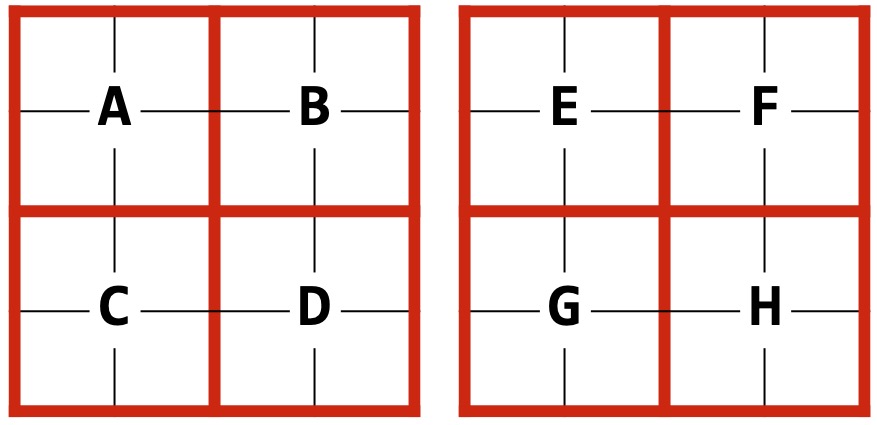
Rather than producing one MinHash for an image, we can produce multiple! Then we can judge the overall similarity of our PNGs based on the fraction of MinHashes about some user-defined threshold of similarity.
In this MP, we will only compare our sketches directly (ex: A to E, B to F, etc…) but there’s nothing stopping us from re-arranging these tiles to identify sub-images in any way we like!
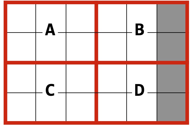
Our images don’t even have to be of a uniform size! When we define a number of tiles (which in our case will always be the same count for both width and height), the actual number of pixels in each tile don’t matter! Here our grey pixels arent in the real image – and we will have to make sure we don’t index out of bounds when building the sketch!
In this example, Given a 5 x 4 pixel image and numTiles=2, I define each tile to be 3x2 in size. This results in a sketch of six ‘pixels’ for both A and C, but B and D only contain four ‘pixels’ total. But I can still use MinHash on each tile to produce a set of four tiles that can be directly compared against the four tiles (E, F, G, H) above!
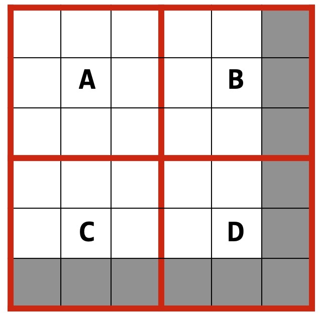
It is up to you to work out the logic for correctly sizing up PNG partitions! Take this 5 x 5 pixel image for example (also with numTiles=2). There is no clean integer split so both our last row and last column will have pixels that don’t exist. Of course, this means the bottom right tile can have significantly less pixels than the rest, but since we’ve already handled the edge case of ‘not having k unique items’ your code should work for any possible input!
To help you work through the math (and as another working example to get you started), given a 8x10 PNG with numTiles=3 we would partition our space into:
width_length = 8/3 = 2.666 (3 tiles of size 3)
height_length = 10/3 = 3.333 (3 tiles of size 4)
For Part 2, you will be writing up a MM (MinHash Matrix) class with the following functions:
MM::MM()MM::getMinHash()MM::countMatchTiles()
Please notice that a significant amount of information is missing from this class. It is up to you to determine how this class is actually implemented. The autograder will only check that the provided functions return the correct values.
Datasets — Part 2
To assist you in debugging your code, a number of randomly generated datsets have been provided. For Part 2, the relevant datasets include:
r_50_100– Randomly generated PNGs of size 50 x 100 (Row x Column)r_500_500– Randomly generated PNGs of size 500 x 500 (Row x Column)twocolor_10_10– Datasets comprised of two colors, each of size 10 x 10 (Row x Column)sixcolor_100_100– Datasets comprised of 6 colors, each of size 100 x 100. (Hopefully by now you understand the syntax)
Each of these directories contains one or more of the following sub-directories. A raw folder contains the PNGs themselves, which your MM constructor will take as input. Most of the directories also contain some pre-computed MinHash sketches, stored in the format <Hash Function>_<Num Tiles>_<Num Mins (K)>. For example hash_1_5_100 implies that these hashes were produced using the provided hash1 hash function, the file was partitioned using a numTiles=5 (so a 5x5 collection of tiles) and each tile is storing the bottom k=100 values. The files are stored from left to right, top to bottom, matching the arrangement of letters in all of the above example images.
Part 3: Representing all MinHash pairs as a Graph
As you observe the MinHash sketch’s accuracy on PNGs (even taking into account we are first reducing color images to black and white), you may be wondering why anyone would use this method at all! If you are unconvinced that being able to convert any size image into a series of numbers is not useful, well maybe you just have to do it more! In Part 3 of this assignment, you are required to write one additional function which, when given a collection of images, computes every possible pairwise comparison of similarity and outputs the results as a weighted graph. This may sound daunting both from a coding (and runtime) point of view, but it’s actually very straightforward (and fast) given your previous code!
The output edge list should be formatted as a vector of size-3 integer tuples (std::tuple<int, int, int>). This is the standard format for a weighted edge list with one modification – instead of storing the vertices of our edge list as strings (the filenames), we are storing them as numbers (the index in the input list). For example:
Given Input List: {"A.png", "B.png", "C.png"}

My edge list might look like:
0 1 5 # A.png and B.png have five tiles >= threshold
0 2 8 # A.png and C.png have eight tiles >= threshold
1 2 9 # B.png and C.png have nine tiles >= threshold
Note a few things in the above example:
- We never bother computing the self-loop edge
{0 0 X}, as we will always have a perfect match with ourselves. - We do not need to compute the edge between B and A (
{1 0 5}) after computing the edge between A and B ({0 1 5}). - Edge weights are the total number of tiles that are above some threshold (one of your input arguements) NOT the fraction of tiles which are above that threshold. This makes grading easier in case you decide to round in weird ways.
The functions you need to implement for part 3 include:
build_minhash_graph()
Datasets — Part 3
There are no unique datasets for Part 3. You should test your code using the provided random PNGs used in Part 2 but if you are interested in doing something fun or creative, consider trying out the datasets you used for tiles in mp_mosaics. For your convenience, I’ve copied the relevant suggestions here:
- Use the UIUC IGram dataset:
uiuc-ig.zip. - If you have an Android, Google Photos usually backs up your photos to the cloud at photos.google.com. You can download them as a ZIP file.
- If you have an iPhone, Apple usually backs up your photos in iCloud. You can download them as a ZIP file.
- Using a computer and a bit of time, you can download a bunch of your photos from Facebook, Instagram, Twitter, etc.
Grading Information
The following files are used to grade mp_sketching:
src/sketching.cppsrc/sketching.h
All other files will not be used for grading.