Posted: June 20th, 2015
Due Date:9:00 P.M., Friday July 10, 2015
You've been hired by the eccentric toymaker and party supplier Mr. Funnstuph of Kansas City to build a monument to his greatness. The monument will be built in Kansas City Missouri. Being the eccentric man that he is, and having not done particularly well in his Physics classes in college, Funnstuph has decided that the best testament to his glory would be a structure composed of his two best-selling items, Slinkys and Happy Helium Balloons. He wants you to build an arch composed of Happy Helium Balloons attached between equal-length Slinkys.
Knowing Slinkys to be way too floppy for your task, you make a desperate attempt at practicality:
"Mr. Funnstuph, I think your monument will be even more... glorious if we use specially made Slinkys."
"Oh? What kind of Slinkys should I use?"
"Well, the structure would look more imposing if you use especially thick Slinkys, and you vary the thickness."
"A brilliant idea! What do you call these modified Slinkys?"
"Springs, sir."
"Springs! What an intriguing label! Seems a little bland, though. Maybe we can market these as some Slinky variant. Springument? Splinky? No, no, how about Monusplink?"
"..."
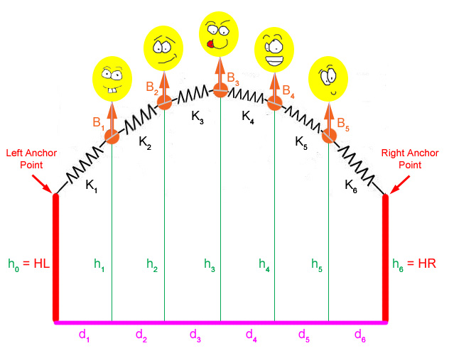
The purpose of this machine problem is to find spring constants Ki for i = 1, 2, ..., N+1 springs that connect in series with N balloons (see figure below). Every spring should be stretched to an identical length. The computation proceeds by modifying the spring constants Ki so that all the spring lengths are length L/(N+1), L being the total length of all N+1 springs when the system of springs and balloons reach their equilibrium state. The two ends of the system are attached to left and right anchors with heights HL and HR, respectively. We will also find the x and y positions of the attach points of the balloons to the springs and plot the system using MATLAB. Figure 1 shows a system with five balloons. However, your program should handle any number of balloons, not just five, along with anchors of different heights.
Note that realistically (or as realistic as you can get with a monument made with Slinkys and Happy Helium Balloons), the balloons should be attached to the springs but float above the springs. We will be using the point of attachment of the balloons in the calculations, not the balloons themselves, to simplify the calculations. Also, the values Bi for the balloons reflect their lifting force after gravity is factored in, not their gaseous volume or anything complicated. For the purposes of the lab, consider the balloons to be a single point of upward force on the arch between springs, not the bags of gas that they actually are...
Figure 1.
There are 6 tasks that you need to complete in this part:
Write a main function. Note that main returns a value.
Write a function find_d
that computes a vector d of horizontal distances between
successive balloons from a vector K of spring constants:
d = [d1 d2 d3 ... dN+1]
is of length N+1 (where N is the number of balloons in the
system)
and
K = [K1 K2 K3 ... KN+1]
is also of length N+1.
Write a function build_Xvec that builds a row vector of length N+2, which starts with the x-position of the left anchor, followed by x-positions of the balloons, and ending with the x-position of the right anchor.
Write a function find_h that builds a
row vector of length N, of the y-coordinates of the
balloons:
y = [y1 y2 y3 ... yN]
is of length N.
Write a function build_Yvec that builds a row vector of length N+2, which starts with the y-position of the left anchor, followed by y-positions of the balloons, and ends with the y-position of the right anchor.
Write a function spr_length that computes a vector of spring lengths from the vectors of x-positions and y-positions of balloons padded with the anchor points.
More detailed instructions and specifications will be given in later parts of this handout.
The data characterizing the system are provided in the file mp1_data.m.
The file contains the following variables:
N: The number of balloons used in the system
L: The total length of all springs.
K: A row vector containing the spring constants (Length: N+1)
B: A column vector containing the balloon forces used in the system (Length: N)
HL: The height of the left anchor point
HR: The height of the right anchor point
D: The total distance -- The (horizontal) distance between the left and the right anchors
Important Note: The names for all the functions and variables are case-sensitive, so make sure your functions and variables are named exactly what we specify here!
Before you start working on the project make sure you have a good understanding of materials covered in lectures 3-6, lab activities 3 and 4, and sections 3.1, 3.2, 4.1, 4.2, and 5.1 of Getting Started with MATLAB.
In order to avoid unexpected errors due to incompatibilities between different versions of MATLAB, please use only MATLAB 7.0 or higher for editing, debugging and checking your programs with the checker.
Copy mp1_data.m and mp1demo.p into your home directory. You can run the demo program by typing mp1demo at the MATLAB prompt. The demo program demonstrates how your program should run. It solves the system using mp1_data and makes a plot of the system. You can use the demo to compare your graphs for Parts 1 and 2 (but not Part 3). After you finish coding, you can run your own program by typing main at the MATLAB command prompt.
After opening MATLAB, run the mp1_data script by typing mp1_data at the MATLAB prompt. After running the script, check to make sure that the variables N, L, K, B, HL, HR, and D have been defined for you to use in MATLAB. Feel free to modify the values in mp1_data to test if your program can handle varying values.
We have provided a checker program for you. In order to run the checker, type mp1_check at the Matlab prompt. The checker has a menu where you can select which function to check (of course you must have completed the function first). Always check and verify each of your completed functions before moving on to the next.
This section explains the math you need to construct and solve the system of equations. Please make sure you understand the material covered in this section. Some of equations derived in this section will be referenced later when you write your code.
Remember the required calculations are:
Calculate the vector of horizontal distances, d, between successive balloons from the vector of spring constants K.
Calculate the vector of the heights (y-positions) of the balloons.
Calculate the vector of spring lengths.
Update the vector of spring constants, K, according to the spring length vector as expressed above.
First, focus on only one balloon Bi in the system:
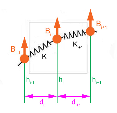
Figure 2.
Derive equations for solving horizontal force and the values of the distances between successive balloons
a) At any point in the system, the force acting on a spring can be decoupled into the force in the x direction (HF, horizontal force) and the force in the y direction (VF, vertical force). To calculate the values of the distances between each balloon, we only need to consider the force acting in the x-direction, which is HF (horizontal force). To calculate the values of the heights of the balloon bases, we only need to consider the force acting in the y-direction, which is VF (vertical force).
b) From the equations below, we can compute the value of HF and the values of the distances between each balloon:
 ......... equation_0
(D equals the sum of the values of distance between each balloon)
From Hooke's law, we can conclude:
(Horizontal force only concerns the displacement in x-direction. Since the system is in equilibrium, the horizontal force is the same throughout, which we denote as HF.)
Divide both sides of the above equation by Ki,
 ...........
equation_1
...........
equation_1
Go back to equation_0
and substitute di with .
.
 (Substitute di
with)
(Substitute di
with)
 (Move HF
out of summation)
(Move HF
out of summation)
 ............ equation_2
(Divide both sides by
............ equation_2
(Divide both sides by )
)
Substituting the value of HF, as obtained from equation_2, into equation_1, we get
 ............
equation_3
............
equation_3
(Note: Given D and vector K, we can solve for vector d using equation 3)
Derive equations for the values of the heights of the balloons
To calculate the heights, only forces acting along y-direction are concerned. The equilibrium condition for each balloon force Bi is given by:
These equations define a tri-diagonal system of linear equations for the heights h1 to hN of the balloon forces B1 to BN. Note that h0 is the given HL while hN+1 is HR. We solve the system by solving the matrix equation
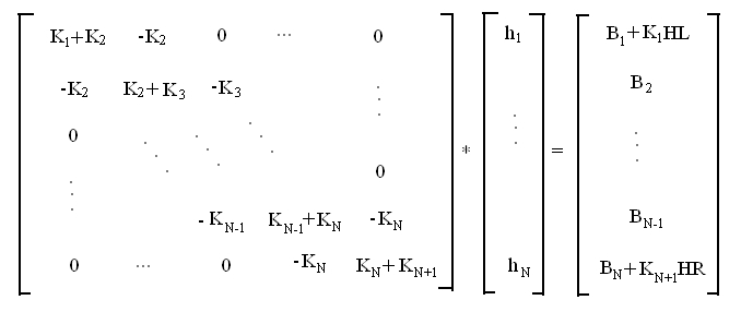
which can be expressed concisely as
for a matrix lhs and a column vector rhs.
The following equation can be used to solve for h, which represents the values of the heights of the balloons:
 ........ equation_4
Please check lab activity 4 for more detailed information.
Derive equations for the spring lengths
You need to solve for the length for each individual spring in the system. Given two points (a, b), (c,d) on a plane, the distance between these two points is
You can use the same equation to calculate the lengths of springs. Instead of using two points, use two vectors, as shown below. One vector represents the x-positions of all the points. The other vector represents y-positions of all the points. For more information, please check out lecture 5, slide 11-27.
len = sqrt(diff(x).^2 + diff(y).^2) ........... equation_5
4. Implementation
You have to create six files: main.m, find_d.m, build_Xvec.m, find_h.m, build_Yvec.m, and spr_length.m. All the files, including main.m, are MATLAB functions. The main function calls other functions in order to calculate the final solution needed for this MP.
The table below summarizes the functions that you need to write, the files to store them, and the operations for each function.
|
Name of function |
Store in file |
Function operation |
|
find_d |
find_d.m |
Computes the values of the distances between the balloons (Step 2) |
|
build_Xvec |
build_Xvec.m |
Builds a row vector, which contains x-positions of the left anchor point, the joint points (where the balloons attach), and the right anchor point. For plotting purposes. (Step 3) |
|
find_h |
find_h.m |
Computes the values of the heights of the balloons (Step 4) |
|
build_Yvec |
build_Yvec.m |
Builds a row vector, which contains y-positions of the left anchor point, the joint points, and the right anchor point. For plotting purposes. (Step 5) |
|
spr_length |
spr_length.m |
computes the length of each spring. (Step 6) |
This section describes how to implement the above functions in a step-by-step fashion. We start with main.m, then implement each of these functions. Finally, we return to main.m to complete the whole program. You will not be able to check your entire program (excluding the extra credit) until you complete Step 8.
Make sure you use exactly the same file names as what we specify here.
Important: Make sure each command line in your functions ends with a semicolon (to suppress the output). You could remove a semicolon to see some intermediate output for debugging purpose - but remember to add it back before you submit your final code.
Create a file called "main.m" in your home directory. Add the following lines to your main.m file:
function handles = main()  % main is a function
clear all;   % clear variables
close all;   % close all open figures
clc;         % clear screen
mp1_data;    % load data file
Then you have to fill "main.m" with function calls to functions that you are going to write:
d = % function call to find_d (Step 2)
X = % function call to build_Xvec (Step 3)
h = % function call to find_h (Step 4)
Y = % function call to build_Yvec (Step 5)
len = % function call to spr_length (Step 6)
From Step 2 to Step 6, at each step, you need to add a line of function call in "main.m". (Note: for more information on how to make a function call, please check section 4.2 in Getting Started with MATLAB and lecture 2). At the same time you must implement the function that is being called and put the function code in the corresponding file. The order you call each function should be exactly the same as specified above. The result (output) of each function is stored in a variable. For example, the result of "find_d" is stored in a variable (which is a vector) "d". We shall edit "main.m" in step 7 to create a loop. Finally, in step 8, we will create the code for plotting the solutions.
Write a function called "find_d" and store it in file "find_d.m".
This function solves the values of the horizontal distances between each balloon (using equation_3). It accepts 2 parameters "D" and "K" (in this order). It returns a row vector of the values of the distance between each balloon. In "main.m", write a function call to "find_d" and store the return value in a vector called d.
Write a function called "build_Xvec" and store it in file "build_Xvec.m".
This function builds a row vector that contains the x-positions of the left anchor point, the balloons, and the right anchor point in the system. It accepts a single parameter "d". Using the MATLAB built-in function cumsum, calculate the x-positions of the balloons and the right anchor using d and store them in a vector called "sub_x". Then, you can build a new vector by appending the x-coordinate of the left anchor (which is 0) to the front of sub_x. Your function should return this new row vector. In "main.m", write a function call to "build_Xvec" and store the return value in a vector called X (capitalized).
The reason for building a vector that has the form of
[x_position_of_left_anchor_point x_positions_of_weigths x_position_of_right_anchor_point]
is that we need to plot the graph of the system in the latter step of the project. The above provides all the x-coordinates needed to plot the system.
Write a function called "find_h" and store it in file "find_h.m". This function computes the value of the heights of the balloons in the system. It accepts parameters "K", "B", "N", "HL", "HR" (in exactly this order), and returns a row vector of the balloons' y-positions. Fill in the code for solving the heights of the balloons. Note: you should have already written this function in lab 4.
In "main.m", write a function call to "find_h" and store the returned solution in a row vector called h.
Write a function called "build_Yvec" and store it in file "build_Yvec.m".
This function builds a row vector that contains the y-positions of the left anchor point, the balloons, and the right anchor point in the system. It accepts parameters "HL", "HR", and "h" (again, in this order). You build a new vector by appending the y-coordinate of the left anchor point (HL) to the front of h and the y-coordinate of the right anchor point (HR) to the end of h. Your function should return this new row vector. In "main.m", write a function call to "build_Yvec" and store the return value in a vector called Y (capitalized).
The reason for building a vector that has the form of
[y_position_of_left_anchor_point y_positions_of_balloons y_position_of_right_anchor_point]
is for plotting the graph of the system. The above provides all the y-coordinates needed to plot the system.
Write a function called "spr_length" and store it in a file called "spr_length.m". This function computes the length of each spring using equation_5. It accepts arguments "X" and "Y" (saved results of Step 3 and Step 5), and returns a row vector of spring lengths.
In "main.m", write a function call to "spr_length" and store the return value in a variable called len.
Now we need the program to keep adjusting the spring constants K until all the spring lengths are equal to L/(N+1) (our desired solution). To do this, we'll use a while loop. A while loop takes a boolean expression, and if the expression is true, the code statements between while and end are executed. The program then jumps back up to the boolean expression and evaluates it again, then repeats the process. Thus, while the expression is true, the code statements in the loop's body keep running. Type "help while" at the MATLAB prompt for more information. While loops are also covered in section 4.3 in Getting Started with MATLAB.
Modify your code as shown below by adding the while loop, the code to modify K and calculate error (to be explained below). Newly added parts are shown in bold.
function handles = main()
clear all;
close all;
clc;
mp1_data;
error = 1;
while error > 1.0e-5
  d = % function call to find_d (Step 2 )
   X = % function call to build_Xvec (Step 3)
   h = % function call to find_h (Step 4)
   Y = % function call to build_Yvec (Step 5)
   len = % function call to spr_length (Step 6)
   % calculate error here
      _________________________________________________

   if error > 1.0e-5
      % modify K here
        _______________________________________________
   end
end
We need to modify K during each iteration of the loop, using the following formula:
Intuitively, we're multiplying each spring constant by the ratio of the current length to the target length of L/(N+1). Springs that are too long will be made stiffer, while those that are too short will loosen.
We need to decide when to stop the loop - when we are close enough to our desired solution. To achieve this, we calculate the error of the current solution, which is the sum of the difference between each spring length and the target length:
We'll initially set error to 1, just to make sure the loop runs the first time (otherwise the program may just skip the loop completely). The condition for the loop to exit will then be when the error is equal or smaller to 1.0e-5 (a very small value).
Hint: You may use abs function.
Once the loop is finished, all the spring lengths should be very close to L/(N+1), and we are done.
Now you have solved the problem correctly, you should complete the last task by making a plot of the system. Add some code to plot X and Y in "main.m", between the call to spr_length and the code to modify K. Mark the location of each balloon with a point dot and connect the balloon locations with solid blue line. Note that the command to make the plot using a line with points at the joints is somewhat tricky; if you have the wrong order for the plot formatting commands, MATLAB will think you want to plot a dotted line instead. The preferred order for plot style is color then pointstyle then linestyle. See the lecture notes or try help plot to learn the symbols for the different styles.
(For more information regarding to MATLAB plot function, refer to section 6.1 from Getting Started with Matlab or type "help plot" at the MATLAB prompt.)
Note that the result of the call to the plot function is first assigned to the temporary variable h1. And then, after the loop, h1 is assigned to the first element of the return vector handles. It is necessary in order to check the correctness of your plots. If you skip this assignment your plot will be graded incorrectly.
To make sure that the spring lengths visually look like they're equal length, use the command axis equal after your plot command. This makes the aspect ratio of the figure equal.
Also, we'll add a pause of a tenth of a second to make sure each separate plot is visible.
Your loop should now look like this:
error = 1;
while error > 1.0e-5
   d = % function call to find_d (Step 2 )
   X = % function call to build_Xvec (Step 3)
   h = % function call to find_h (Step 4)
   Y = % function call to build_Yvec (Step 5)
   len = % function call to spr_length (Step 6)
% fill in the blank below with the command to plot system with blue lines and points
h1 = ________________________________________;
axis equal
pause(0.1)
% calculate error here
________________________________________________
if error > 1.0e-5
% modify K here
________________________________________________
end
end
% this is necessary to check the plots
handles(1) = h1;
% handles(2) is needed for the extra credit, so it is 0 for now
handles(2) = 0;
Save your main.m and run it at the command prompt by typing,
main
If all works well, you should see a plot of an arch that
gradually adjusts its position until it finds a position
where all spring segments have equal length. Run the checker
by typing,
mp1_check
If your arch doesn't converge, what should you do?
To stop your program, press Ctrl-C (Hold the control key and press c). If you are running the checker when you do this, you may need to change your current directory back to your home directory (at the top of the Matlab window).
See if you have any of the following common problems:
Using K(N) instead of K(N+1) in find_h.m when setting B(N).
Forgetting parentheses around N+1 in the formulas for error or K in main.m
Now we're going to perform a little optimization. Notice that the coefficient matrix we create to solve the system of equations in find_h can have a lot of zeroes if there is a large number of weights. This can bog down calculations, because MATLAB will spend the time to use each of those zeroes, even though they don't do anything, and they also take up space because MATLAB stores them as part of the matrix. The solution to this is to use something called a sparse matrix. Sparse matrices store only the non-zero elements; all other elements are assumed to be zero. This saves on storage space for matrices with lots of zeroes, and it also speeds up computation, since MATLAB will simply ignore the non-existent zeroes in the sparse matrix when doing matrix multiplication.
To create sparse matrices, we'll use the command "spdiags", which will replace diag. spdiags is a tad more complicated (but more powerful) than diag. The format for using spdiags is spdiags(D, c, m, n), where:
D: matrix containing the diagonal columns.
c: "control vector" of diagonal positions. c has as many elements as D has columns.
m: number of rows in resulting matrix.
n: number of columns in resulting matrix.
That is, spdiags will take each column of the D matrix and place it on the diagonal indicated by the control vector in an m x n sized matrix. Here's an example of how it works. First, we construct a matrix with the diagonal columns:
>> D = [1:5; 6:10; 11:15]'
D =
     1     6    11
     2     7    12
     3     8    13
     4     9    14
     5    10    15
Note the three columns of D. We're going to use the columns as diagonals in a 5 x 5 matrix:
>> A1 = spdiags(D, [0 1 -2], 5, 5)
A1 =
   (1,1)        1
   (3,1)       11
   (1,2)        7
   (2,2)        2
   (4,2)       12
   (2,3)        8
   (3,3)        3
   (5,3)       13
   (3,4)        9
   (4,4)        4
   (4,5)       10
   (5,5)        5
Yes, A1 is actually a matrix. This is how MATLAB displays sparse matrices, as a list of indices with their values. Any index location in the matrix that isn't listed above, like A1(1,3), is implied to be a zero. However, this isn't a particularly good format for viewing the matrix, so let's multiply A1 with an non-sparse identity matrix to force it into the standard matrix format:
>> A2 = A1 * eye(5)
A2 =
     1     7     0     0     0
     0     2     8     0     0
    11     0     3     9     0
     0    12     0     4    10
     0     0    13     0     5
A2 is the same matrix as A1, except in non-sparse form. How did the columns of D turn into the diagonals of A2? Let's break it down some more, using the same data as above:
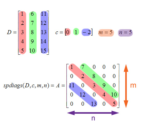
Figure 3.
Given D, c, m, and n, the resulting matrix A from spdiags is of m x n size. Each column of D is used to create a new diagonal. The first column is on the main diagonal of A, the second column is on the first upper diagonal, and the third column is on the second lower diagonal. How did they get there? Note the control vector c: 0 for the first value, corresponding to the main diagonal, 1 for the second value (first upper diagonal), and -2 for the last value (second lower diagonal). Thus, the c vector controls which diagonal the columns of D appear in A.
But wait, you may (should) be saying. How do the diagonals get created if the column of D isn't the same size as the diagonal it's being used for? How did the second column of D end up on the first upper diagonal of A if the column has five elements to the diagonal's four? The solution is that MATLAB will drop values from the D columns to make the diagonal fit. In the case of upper diagonals, the values are dropped starting from the top of the column matrix. Thus, the 6 from the second column of D was discarded, and 7 through 10 were used to make the diagonal. Similarly, in the case of lower diagonals, values are dropped starting from the bottom of the column matrix. For the second lower diagonal, 14 and 15 were dropped, while 11 through 13 were used.
Now let's put all that newfound knowledge of spdiags to good use. Create a new function called "find_h2" and store it in a file called "find_h2.m". This function will take the same parameters as find_h, in the same order. You can copy most of the code over from find_h. The constants vector remains unchanged and the calculation to find the h values remains unchanged. However, instead of using multiple "diag" calls to create your coefficients matrix, now you will use a single call to "spdiags" to create a sparse version of your matrix. That is, make your own columns matrix and control vector, then feed them to spdiags along with the appropriate values for the matrix dimensions to get the same coefficients matrix as before, but in sparse form.
Now, change main.m to use find_h2. Comment out the line for find_h (put a "%" in front of it), and put a new line under it that calls find_h2 and assigns the result to h.
error = 1;
while error > 1.0e-5
   % some function calls here
   % h = commented-out call to find_h
   h = % call to find_h2 here
   % your call to spr_length here
   % command to plot system with blue lines and points
   axis equal
   pause(0.1)
   % modify K here
   % calculate error here
end
% this is necessary to check the plots
handles(1) = h1;
% handles(2) is needed for the extra credit, so it is 0 for now
handles(2) = 0;
If you'd like to test how the sparse matrix affects calculation speed, modify your mp1_data file and set N to some high number (say, 1000). Try running main with both find_h and find_h2 (commenting out one or the other in main.m). You'll notice a significant slowdown with find_h compared to find_h2.
When handing in your solution, make sure that find_h is commented out (not deleted, since we want to see that you called it in part 1) and that find_h2 is the function that your main.m is calling.
After doing endless tinkering with the springs and balloons,
you've finally found a configuration of the arch in Kansas
City that Mr. Funnstuph thinks is pleasant. But wait! Could
the well-known arch of St. Louis Missouri be exactly the same
shape as Mr. Funnstuph's arch?
The mayor of St. Louis has sent you a copy of their top-secret formula to create their arch, so you can compare to your arch and see if they're the same. Modify mp1_data to use Mr. Funnstuph's preferred numbers:
L=90
N=5
B = 5*ones(N,1)/N
HL = HR = 10
D=30
K = 5*ones(1,N+1)
The shape of the arch in St.
Louis is defined by the equation of a reversed catenary curve:
 (equation_6)
where  is a horizontal tension, and
 is a weight of one foot of the curve, depending
on the material from what the arch is made.
is a weight of one foot of the curve, depending
on the material from what the arch is made.
For the right and left anchors of Kansas City arch this equation looks like:
where
 and
and  are
horizontal coordinates of the left and right anchors relative
to the midpoint of the arch,
are
horizontal coordinates of the left and right anchors relative
to the midpoint of the arch,  . Subtracting
  from
from  and
dividing both parts of the equation by
and
dividing both parts of the equation by  we get:
since
 , the right-hand side can be
rewritten as:
, the right-hand side can be
rewritten as:
 (equation_7)
The length of the curve can be determined by the following expression:
where:
Therefore
 ,
,
Dividing both sides of the
above equation by  , we get:
 .
(equation_8)
.
(equation_8)
Since  , equation 7 can be rewritten:
 (equation_9)
Dividing both sides of equation 7 by equation 9:
Since  , the second term of the right-hand
side of equation 7 can be rewritten as:
, the second term of the right-hand
side of equation 7 can be rewritten as:
 , so the whole equation 7 looks
like:
, so the whole equation 7 looks
like:
 (equation_10)
Replacing  with t
, we define the function f(t) as follows:
with t
, we define the function f(t) as follows:
 (equation_11)
2. Implementation
Write a function called stlouis_aux that takes an input parameter t and computes the value f(t) from equation 11 above, where XR = D, and XL = 0. Note, that you should call mp1_data script in the first line of the function stlouis_aux in order to obtain values for HR, HL and L.
Next write the function called stlouis, which plots the catenary curve defined by
where in equation 11 we defined
t =  . The first twos lines of this function is,
function h2 = stlouis()
mp1_data;
hold on
We will have to first compute values t =W/T , XC and A. As in
parts 1 and 2, function stlouis should return the result
of calling the plot function to plot the catenary
curve. In order to plot the graph, you need to compute the
following values:
1. In equation 11 we defined t = . We can find t by solving the
equation f(t) = 0 for t ( f(t) is defined above; use fzero
with an initial guess of .1). Note that we named the function f
, stlouis_aux in our code in step 1.
2. Once we know t we can then solve for XC by using the formula,
3. Knowing both t and XC we can
now solve for A,
4. Plot the catenary in red
using the equation where x is a vector of 100 evenly
spaced values between 0 and D and assign the result of
calling the plot function to the output parameter of stlouis.
h2 = plot(....);
Change the last line of the main function from:
handles(2) = 0;
to
handles(2) = stlouis;
to see if the arches match. Run your program by typing
>> main
at the Matlab prompt. Chances are they are not quite the same...
Mr. Funnstuph: "Ha! It's not the same at all!"
You: "But sir, we're only using this number of balloons as a test. The real arch uses many more balloons. We're just not using enough data points..."
Mr. Funnstuph: "Shh! Be quiet!"
Now modify your mp1_data and set the number of
balloons to 100 (N = 100). Run main
and stlouis
again and see how close the arches are.
Mr. Funnstuph: "Oh, shoot."
Looks like Mr. Funnstuph can't make his monument of toys after all. We're going to have to confiscate all the materials...
Before you hand over your programs, though, make sure that each file has your name and section as a comment at the top of the file. Also, provide enough comments to make the program understandable. This means comments on the purpose of each function or script, including what they take as input and what they return as output. This should be done for functions as helpful information directly below the function definition line (see Lab 3, Section C for more details). Scripts can just have comments for major sections. Note that the comments should be an overview and explanation, not a line-by-line recap of the program (so comments that are twice as long as the function are bad). Please don't try to comment every line of code.
Everything working perfectly (correct answers and graph plotted right) = 50 points. The grading is based on a per function basis. Each function is graded on an all or nothing basis. The table below lists points per function.
|
Function |
Points |
|
find_d |
5 |
|
build_Xvec |
6 |
|
find_h2 |
7 |
|
build_Yvec |
5 |
|
spr_length |
5 |
|
main |
15 |
|
comments |
7 |
|
Total (w/o Extra Credit) |
50 |
|
stlouis, stlouis_aux |
9 |
|
comments |
1 |
|
Total (Extra Credit) |
10 |
Click here for handin
instructions.
That's it! You're done!
 (Aww, you don't want to play with the balloons
anymore?)
(Aww, you don't want to play with the balloons
anymore?)