Compute the
volume by running the function named 'vol'.
When using 'vol',
we must specify a box that contains the object we're
measuring. We'll get the best results if we use the
smallest box which contains the object. In our case, the
range of the smallest box which contains our ellipse is:
| x
from -1 to 1 |
| y
from -1 to 1 |
z
from -2 to 2
|
Make sure to enclose 'inEllipse' in single
quotes when using it in the call to 'vol'.
- Answer
Part 1: Questions 1 through 3 on your answer
sheet.
How does your answer compare to the analytical answer
given at the beginning of this part?
- Answer
Part 1: Question 4 on your answer sheet.
Part 2: Adaptive Integration.
Instructions:
In this portion of the MP, we will be writing MATLAB code
to compute the definite integral

using the recursive method called adaptive
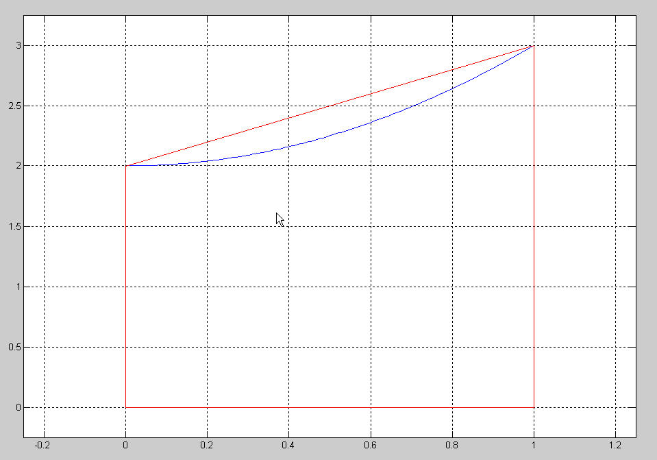
integration. First we use the trapizoidal rule to
perform the integration over an interval [a,b], for a given
function y=f(x). For example see the figure below that shows
a trapezoid with A_approx = (1/2)*(f(a)+f(b))*(b-a) =
(f(0)+f(1))/2 where a = 0 , b=1 and f(x) = x2+2.
If the difference between the true area A and the
area in the trapezoida A_approx is small we are done.
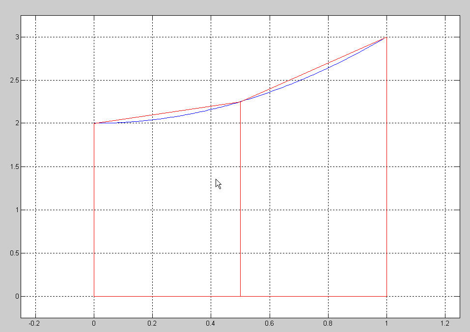
But if we don't know A then how can we know that A_approx is
good? One way to test our approximation is to subdivide the
x axis into two intervals [a (a+b)/2] and [(a+b)/2, b] (or
[0 1/2] and [1/2 1] in our probleam) and form two trapezoids
(as shown in the figure below).
Our method is to compare the sum of the areas of the left
trapezoid and the right trapezoid AL_approx +
AR_approx with the area of the single trapezoid
A_approx and if the difference is small then we are done. If
the difference isn't small then we will use recursion
applied to AL and AR respectively.
We are now going to write a pair of functions to compute
definite integrals!
Open a new editor window by typing the command:
>> edit adaptive.m
Copy and paste the following code into a file called adaptive.m
function area = adaptive(fcn, a, b,N,axis_vec,tol)
% function area = adaptive(fcn, a, b,N,axis_vec,tol)
% Integrate the function y = fcn(x) on the interval [a,b] using N points and the trapezoidal rule.
% axis_vec is a vector [xmin xmax ymin ymax] that sets the size of the graph in the figure window.
hold on
x = linspace(a, b, N);
y = feval(fcn, x);
x2= [a,x,b];
y2 =[0,y,0];
fill(x2,y2,'g')   % the fill command fills a polygon in the plane. The closed region contains the points (a,0) and (b,0)
% 'g' stands for green
axis(axis_vec)
pause(.3)
A = trapz (x, y);   % compute the Area using the trapezoidal formula
x = linspace(a, (a + b)./2, N);
y = feval(fcn, x);
AL = trapz(x, y);  % compute the area on the left half of the interval.
x = linspace((a+b)./2, b, N);
y = feval(fcn, x);
AR = trapz(x, y); % compute the area on the right half of the interval
if abs(((AR + AL)-A)) < tol  % if close enough done so assign output variable 'area' and fill the area in with red
    area = ________________________________;% assign correct value to area
    fill(x2,y2,'r')
    axis(axis_vec)
else  % else we haven't satisifed the tolerance set by the user so compute the area of the left half and add the area
        % computed by the right half.  Fill in the blanks with recursive calls. You will have two calls to the function
          % adaptive.

    area = ________________________________________________________; % use recursion to sum areas between a , (a+b)/2 and (a+b)/2 and b.
end
Answer Part 2:
Question 1 on your answer sheet.
Now, let's test it! At the Matlab prompt try running the
commands:
>> close all
>> format long
>> area =
adaptive(@(x)sin(1./x).^2./x.^2,1/(30*pi),1/(10*pi),925,[1/(30*pi)
1/(10*pi) 0 10000], 1.0e-10)
Executing the above command may take several minutes.
Answer Part 2:
Question 2 on your answer sheet.
Part 3: Solving the harmonic oscillator problem.
Instructions: In this portion of the MP, we will be
writing MATLAB code to plot the position on the horizontal
axis of a weight attached to a spring assuming the
existence of air friction.
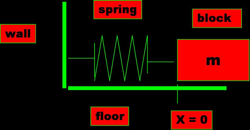
(Think of a spring loaded screen door on your house.)
1. Problem Definition
We will use the Matlab function
ode45. The goal is to plot the horizontal position of the mass
m with respect to time.
2. Refine, Generalize, Decompose the problem definition
(i.e. identify sub-problems, I/O, etc.)
When you code your
solution in the function xvprime.m you should run your
program with the following three cases.
a. m = 1, k = 100, b = 2
b. m = 1, k = 100, b = 20
c. m = 1, k = 100, b = 5
When you submit your
solution you can leave either one of the
three choices listed above.
Assume that at t =
0 , x = 1 and v = 0. Use the time
interval [0, 10].
3. Develop Algorithm (processing steps to solve
problem)
The ODE is described by
the harmonic oscillator:
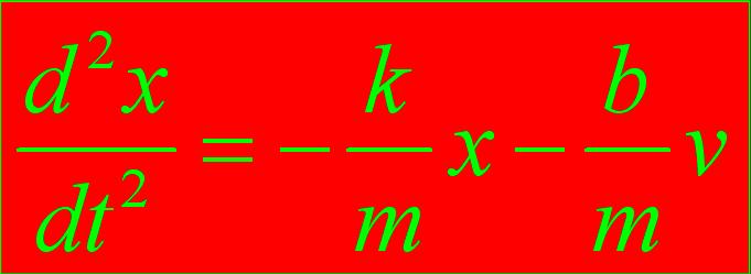
Answer Part 3:
Question 1 on your answer sheet.
4. Write the
Function (Code)
The first
line should be
function xvp = xvprime(t , xv)
%
use m = 1 k = 100 b = 2 as values for now then after you
have done a plot then change b = 20 and later b = 5
5. Test and Debug the Code
Answer Part 3:
Question 2 on your answer sheet.
6. Run the Code
After you have run the
code, plot the solution. Do this for each of the three cases
for b = 2,20,5.
Answer Part 3:
Question 3 on your answer sheet.
You will not handin
the plots. Answer
Part 3: Question 4 on your answer sheet.
Part 4: Ray Tracing
Instructions: In this portion of the MP, you will need
to complete a MATLAB function named ray_trace. This function
plots how lights rays reflect off of a surface of a mirror. We
will assume that light travels in a straight line and will not
consider any effects due to diffraction of light at the edges
of a mirror. We will also assume that you are familiar
with the Law of Reflection (
http://www.physicsclassroom.com/class/refln/Lesson-1/The-Law-of-Reflection
)
We give you the code below that defines the three types of
mirrors we will study. Please copy/paste these into MATLAB.
The first descibes a mirror with shape given by the function
(x-4)2 + y2 = 16. The function has one
input, a scalar y, and the function returns the x value of the
point
on the circle with the given y value. Also, the function
returns the slope of the line normal(perpendicular) to the
surface at the point (x,y).
function [x, nslope] = circle(y)
% function [x, nslope] = circle(y)
x = 4-sqrt(16-y.^2);
nslope = y./(x-4);
The second descibes a mirror with shape given by the function
(x-4)2 + 4y2 = 16. The function has one
input, a scalar y, and the function returns the x value of the
point
on the ellipse with the given y value. Also, the function
returns the slope of the line normal(perpendicular) to the
surface at the point (x,y).
function [x, nslope] = ellipse(y)
% function [x, nslope] = ellipse(y)
x = 4-sqrt(16-4.*(y.^2));
nslope = 4.*y./(x-4);
The third descibes a mirror with shape given by the function x
= y2 / 4. The function has one input, a scalar y,
and the function returns the x value of the point
on the parabola with the given y value. Also, the function
returns the slope of the line normal(perpendicular) to the
surface at the point (x,y).
function [x, nslope] = parabola(y)
% function [x, nslope] = parabola(y)
x = y.^2 ./ 4;
nslope = -y./2;
We will restrict the y values to be on the interval [-1,1].
We will only consider the left hand parts of the circle and
ellipse and only part of the parabola. In reality an actual
mirror is 3D but can be considered as a rotation of the above
functions about the x-axis.
Lastly, we give you an incomplete function named ray_trace.
Please copy/past this function into MATLAB.
function ray_trace(func)
% function ray_trace(func)
% plot surface of mirror
y = linspace(-1,1,100);
[x,nslope] = feval(func,y);
plot(x,y)
axis([-0.5,4,-1,1])
grid on
hold on
% plot horizontal incoming rays and their reflection
% off the surface
% All of your code goes inside this for loop
for y = -1:.25:1
[x,nslope] = feval(func,y);
% plot incoming ray starting at point (4,y)
pointing back horizontally
% to the left
% 'color' [a b c] specifies amount of [red
green blue]
% scale = 0 means that
quiver(x,y,u,v,scale) plots an arrow starting
% at the point (x,y) and in the
direction of the vector (u,v), whereas
% scale = 0.5 would produce a vector
half as long as (u,v)
scale = 0;
quiver(4,y,x-4,0,scale,'color',[0 0 0])
% Comment out the next two lines when you
have completed your code.
% This command plots the normals to the
mirror.
% The rule for reflection is that the angle
between the incoming light
% ray and the normal should be equal to the
angle between the reflected
% light ray and the normal.
% test plot normal
scale = 10;
quiver(x,y, 1, nslope,scale, 'color', [0 1
0])
%plot reflected ray
scale = 0;
%your code goes
here.......................................................................................................
end
Test the above code by typing the following at the MATLAB
prompt:
>> ray_trace('circle')
>> ray_trace('ellipse')
>> ray_trace('parabola')
and note that you shoud see incoming light rays (in black
color) coming from the left of the screen. Light waves from
stars is effectively parallel. We arbitrarily chose a certain
number of incoming rays. We could have chose more or chose
less. You will also see green lines in your figure window.
These lines are normal (perpendicular) to the surface where
the incoming (black) ray struck the surface. The green rays
are not really needed but may be useful as a check for you.
Your goal is to use the MATLAB quiver function to
plot reflected red rays from the point on the mirrors suface
to where the red rays cross the x-axis.
You can use the MATLAB help facility to learn more about
the quiver
function. You can also see how the quiver function has
already been used in the ray_trace function.
Here are a few hints if you need them.
Pick a point (x,y) on the surface of the mirror where
the incoming ray (black) is to be reflected. If the angle
between the incoming ray (black) and the normal to the surface
(green) is named theta then the angle between
the reflected ray (red) and the normal to the surface (green)
must also be equal to theta by the law of
reflection. But the tangent (MATLAB tan
function) of theta is the slope of the
green line (since the black rays are always horizontal). We
have already computed the slope of the green ray as nslope,
so tan(theta)
= nslope. But we want to solve for theta
so use the MATLAB atan function. Now observe
that the slope of the reflected rays (red) is equal to the tan
of twice theta. Write down the MATLAB
code in the ray_trace function and assign
this value to a variable named rslope (short for
reflected slope). Now all you need is one more line of MATLAB
code and you are done. Call the quiver function and
use x, y values that we have just computed to compute a
ray. The color should be red [1 0 0]. You should have,
quiver(x,y,
_____u???______, _______v???_________, scale, 'color', [1 0
0])
but what are u and v ??
Note that (u,v) should be the direction of the reflected ray
(red) and this vector starts at (x,y) and ends where the
reflected ray (red) crosses the x axis . Draw a picture to
figure this out. Your formula will need to use rslope
and y.
Test your code by running the previous tests.
>> ray_trace('circle')
>> ray_trace('ellipse')
>> ray_trace('parabola')
If you have errors then go back to your code for the ray_trace
function.
Once you believe that you have correct results you can edit
the ray_trace function and comment out the lines of code that
create the green lines. Then generate the three figure windows
again but this time when each figure window opens Click on the
menu for the figure window File / Save As and name each
file accodingly. Accept the .jpg extension for each of these
three files.
Submit your file ray_trace.m and Answer Part 4: Question 1 on your answer
sheet.
C'est fini !!!
Your solution to this MP should include the answering the
questions on the Answer webpage ( answer_sheet )and emailing the
answers and all of the following files to
(Jiahui Jiang ta8cs101@cs.illinois.edu).
inEllipse.m
adaptive.m
xvprime.m
ray_trace.m
and the three plots you generated from part four,
circle.jpg
ellipse.jpg
parabola.jpg
