You will need to read the
following instructions in sections 1) thru 3). You will
begin coding in section 4) Implementation
1) Introduction
1.1) Dynamics of Hard Spheres - Your
Honor’s Project
The motion of molecules in a
gas, the dynamics of chemical reactions, atomic diffusion,
sphere packing, the stability of the rings around Saturn, the
phase transitions of cerium and cesium, one-dimensional
self-gravitating systems, a game of billiards or snooker,
front propagation are all examples of dynamics. Also, they
have the additional similarity of having spherical or nearly
spherical colliding objects in each of the above presented
examples. We can take some time here to observe three facts:
1) Their inter-disciplinary nature, 2) The role of Computer
Programming and 3) The fact that a common program written to
simulate the motion of colliding particles can describe all
these phenomena. We could also observe the fact that all these
are at least related to the Brownian Motion
which was introduced earlier.
The purpose of this programming
assignment is to develop a computer program which could
represent to an acceptable level of accuracy, the above
mentioned condition; that is, to simulate the motion of “N”
colliding particles based on
the laws governing elastic
collisions and basic dynamics.
[P.S.: We are really grateful
to the Computer Sciences Department of the Princeton
University for providing us with useful material in this
respect. More information regarding this can be found here.]
2) Modeling
2.1) In General
Modeling refers to the process of the
reproduction of the given problem, usually to a smaller
scale. Modeling often involves certain simplifying
assumptions which make the process of creating a model
simpler.
The modeling involved in dynamical
analysis is in turn sub divided into 2 major steps:-
a)
Creating an Analytical Model
b)
Obtaining a Mathematical Model from the Analytical
Model.
The process of obtaining the Analytical
Model consists of the following main steps:
a) A list
of simplifying assumptions which permit to reduce the real life
problem into a simpler analytical model.
b)
Drawings that depict the Analytical Model.
c) A list
of design parameters.
To create a useful Analytical
Model, you must clearly have in mind the intended use of the
analytical model, that is, the types of behavior of the real
system that the model is supposed to represent faithfully.
Once the analytical model of
the structure has been created, we can apply the concerned
physical laws to convert the dynamical equations of the system
under question into Mathematical equations. These Mathematical
equations so obtained are termed the “Mathematical Model”.
In practice, you will find that
the entire process of creating first an analytical model and
then a mathematical model may be referred to simply as mathematical
modeling.
2.2) Analytical Modeling of the
“Molecular Dynamics” Problem
Any real life problem is a
complex one. However, it is observed that certain simplifying
assumptions can be made which reduce the complexity of the
problem without a great deal of reduction in the accuracy of
the desired variables. In other words, these assumptions make
life much simpler than what it would be otherwise.
For this problem, one major
simplification has been made. The molecule (or the sphere)
under study is an elastic body, which should undergo elastic
deformations upon collisions. However, it has been observed
that neglecting these small deformations does not affect the
end result very much, although it reduces the complexity of
the problem a good deal. So, in the analytical model of this
problem, we assume that atoms or molecules or the spheres
(these three terms are equivalent; the use of any of these
three words in future would represent the same.) in the
container behave as “hard spheres”, also called the “billiard
ball model”. When we focus on the two-dimensional
version of this, they behave as the “hard disc
model”.
We will do our calculations in 2D. (3D would not be much more
difficult but we will leave that for you to do for fun.)
In addition to this major
assumption, we also make other simplifications which result in
the following salient features of this model:
a) “N”
particles in motion.
b) All particles
are confined in the ‘unit box’.
A box of
unit height and width, 0 <= x <=1, 0 <= y <= 1.
c) Particle ‘i’ has the position (rxi, ryi), velocity (vxi, vyi), mass mi,
and radius σi.
d) All particles interact
via elastic
collisions with each other and with the reflecting boundary.
e) No
other forces are exerted. (e.g. no gravitaional effect on particles or
between particles.) Thus, particles travel in straight lines at
constant speed between collisions.
There are two natural
approaches to simulating the system of particles.
A) Time-driven
simulation:
Discretize time into quanta of
size dt.
Update the position of each particle after every dt
units of time and check for overlaps. If there is an overlap,
roll back the clock to the time of the collision, update the
velocities of the colliding particles, and continue the
simulation. This approach is simple, but it suffers from two
significant drawbacks.
First, we must perform on the
order of N2 collision checks per time quantum ,
(actually
N choose 2 particle-to-particle collisions,  = N*(N-1)/2 plus 2*N checks for
the particle-wall collisions).
= N*(N-1)/2 plus 2*N checks for
the particle-wall collisions).
Second, we may miss collisions
if dt
is too large and colliding particles fail to overlap when we
are looking. To ensure a reasonably accurate simulation, we
must choose dt
to be very small, and this slows down the simulation.
We will NOT do time-driven simulation in this MP.
B) Event-driven
simulation:
With event-driven simulation we
focus on those times at which interesting events occur. In the
hard disc model, all particles travel in straight line
trajectories at constant speeds between collisions. Thus, our
main challenge is to determine the ordered sequence of
particle collisions. We address this challenge by maintaining
a event
matrix of future events for each particle. At any given
time, the event matrix contains the next future collision that
would occur for each particle, assuming each particle moves in
a straight line trajectory forever. As particles collide and
change direction, some of the events scheduled on the priority
queue become "stale" or "invalidated", and no longer
correspond to physical collisions. Thus we will have to update
this event matrix. For example, we have the following events
in the queue:
particle# |
time-to-next-collision | particle/wall
1
.02 5 (
particle #1 will collide in .02 seconds with particle #5)
2
.2 1 ( particle
#2 will collide in .2 seconds with particle #1, we haven't
yet taken into account here that particle #1 will first
collide with paricle #5 )
3
.05 -1 ( partice #3 will collide
with the horizontal wall in .05 seconds,
-1 means horizontal wall collision)
4
.4 -2 (
particle #4 will collide with the vertical wall in
.4 seconds, -2 means vertical wall collision)
5
.02
1 ( particle #5 will
collide in .02 seconds with particle #1)
…
N
Inf
-3 ( particle #N
will not make any collisions since a value of -3 means zero
velocity so no collison with
any wall, and there is also no particle collisions. Inf is
the Matlab constant for
+infinity.)
From the values shown above the
next collision for any of the particles is
between Particle 1 and 5 since the time for this collision is
the smallest value ( .02 seconds).
Particle 2’s next collision is with Particle 1 but that won’t
happen since Particle 1 will collide with Particle 5 first ( in .02 seconds).
The event matrix will
have N rows but just two columns (since the first column above
is always 1 thru N we don’t need to store this in the event
matrix.).
So the format of the event
matrix will be such that the i-th
row of the event matrix has the form:
[ time-to-next-collision
j ]
where j is an integer from 1 to
N representing a particle number or -1,-2 representing a
horizontal or vertical wall collision respectively or -3
meaning NO COLLISION with wall or partice.
In the case where j = -3
instead of using the Matlab Inf as in a
row value of
[ Inf -3]
instead we could record this row as
[ arbitrary_real_number
-3]
if we wanted to avoid using the Matlab constant Inf.
3) The Math
In this section we present the
formulas that specify if and when a particle will collide(hit) with the boundary (wall)
or with another particle, assuming all particles travel in
straight-line trajectories.
For simplicity we will avoid considering simultaneous
collisions with 3 or more particles or simultaneous collisions
of separate pairs of particles or a particle that hits the
corner of the box ( hits both
walls simultaneously).
3.1) Collision Prediction
I) Collision between
particle and a wall:
Assume you had only a single
particle of radius σ in the unit box (0 <= x <= 1 and 0
<= y <= 1) where the center of the partice
is located at (rx, ry) and thus σ <= rx <= 1-σ and σ <= ry <= 1-σ ,
with velocity (vx, vy).
The questions we need answered are:
1) Which wall will the particle hit, if any?
2) What is the new position vector (rx', ry')
and new velocity vector (vx', vy') after the collision.
3) How much time does it take to hit the wall Δt?
Here is our strategy for
answering the above questions.
We will answer 3) first then use our results to determine 1)
and then 2) will follow.
To answer question 3) ,
If the inital velocity is zero
i.e. (vx, vy) = (0,0) then the particle would
not move and thus not make contact with a new wall( of course
it could be touching a wall and not moving too but that
doesn't change the fact that the particle will not hit a new
wall). This answers question 1) and
to answer question 2) since vx =
vy = 0 then its new position at
any future time would be (rx', ry') = (rx,
ry) and new velocity (vx', vy')
= (0,0).
Else if the particle were moving, ie. vx and vy
are not both 0 then then there must be a future contact with
the walls of the unit box. Lets solve this problem in a
lazy way. We first assume that the box has no vertical walls,
only horizontal walls (extended infinitly in both directions) and then
try compute Δt_y the time the hit
the horizontal wall. Next assume that the box has no
horizontal walls jut vertical walls and then try to compute Δt_x the time to hit the vertical
wall. Now that we have computed Δt_y
and Δt_x find the smallest of the
two Δt = min(Δt_x, Δt_y)
and that will tell us which wall is actually hit. This answers
question 1). Question 2) is answered by using the formula (rx', ry')
= (rx, ry)
+Δt * (vx,vy) and (vx',
vy') = (vx,
-vy) if a horizontal wall is hit
and (vx', vy')
= (-vx , vy)
if a vertical wall is hit. There is a very rare case
where Δt_x = Δt_y when the particle hits the corner
of the box. You don't have to write code for this case. If you
write code then the new positon is also given by the same
formula (rx', ry') = (rx,
ry) +Δt
* (vx,vy)
but the new velocity is given by (vx',
vy') = (-vx,
-vy).
Yes, it may occur that vx > 0 and vy
= 0 so that computing Δt_y
= Inf in Matlab
but since Δt_x is finite
then Δt = min( Δt_x, Δt_y)
= Δt_x and this is correct
so your code should work correctly without any changes.
Also, it may occur that vx = vy = 0 but this would give Δt = min( Δt_x,
Δt_y) = min(Inf,
Inf) = Inf
and that is correct so again you don't need to modify your
code for this special case. If you don’t like working with Inf then in
these cases set Δt = 1.0e100.
All that is left to do is to
find the formulas for Δt_x and Δt_y.
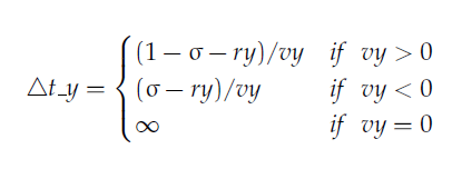
a) Δt_y ---Horizontal Wall Collision
Given the position vector (rx,
ry), velocity vector (vx, vy),
and radius σ of a single particle at time t,
we wish to determine if and when it will collide with a
vertical or horizontal wall. the
new velocity (vx', vy') = (vx,
-vy) for either upper or lower
wall collision. To determine the new position (rx',
ry') consider the
figure below.
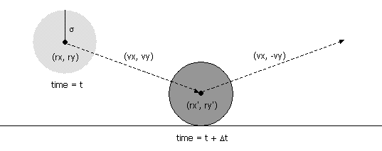
The
figure above shows a future collision of a particle with the
lower horizontal side of the boundary(wall).
A particle comes into contact with a horizontal wall at time t
+ Δt
if the quantity ry + Δt * vy
equals either σ (lower horizontal wall collision) or (1 - σ)
(upper horizontal wall collison).
Solving for Δt
yields:
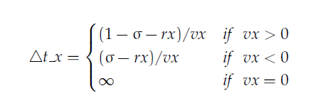
b) Δt_x
---Vertical
Wall Collision
An analogous equation predicts the time of collision with a
vertical wall. The
Since we are going to be
dealing not with just one particle in the unit box it may
occur that before a particle hits a wall of the box the
particle hits (or is hit ... depending on your perspective,
that is, from which particle you view the collision) another
particle. We need to answer the following questions.
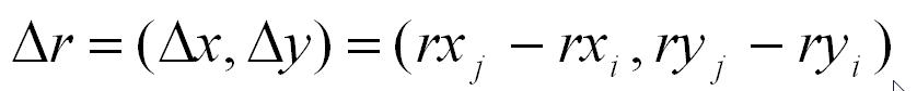
We are given information on
particle i
at time t , its position (rxi
, ryi) and
velocity (vxi
, vyi )
1) Will particle i hit particle j (whose
position at time t is (rxj , ryj)
and velocity is (vxj
, vyj ))
?
2) What is the new position vector (rx',
ry') and new veloctiy
vector (vx', vy')
at the time of collision for both particles i and j ?
3) How much time Δt does it take
for particle i to hit particle j ?
II) Collision between two particles.
Again, we will answer 3) first
and if Δt =
Inf we know there is no collision
but if Δt is finite there will
be a collision and then we will answer 2).
Given the positions and
velocities of two particles i
and j at time t, we wish to determine if and
when they will collide with each other.
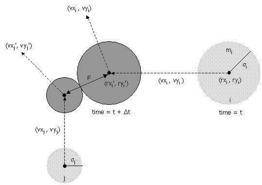
Let (rxi' , ryi'
) and (rxj'
, ryj' )
denote the positions of particles i
and j at the moment of contact, say t + Δt. When the particles collide,
their centers are separated by a distance of σ = σi + σj.
In other words:
σ2 = (rxi' - rxj' )2
+ (ryi' - ryj' )2
During the time prior to the
collision, the particles move in straight-line trajectories.
Thus,
rxi' = rxi
+ Δt
vxi, ryi' = ryi + Δt
vyi EQUATION 1
rxj' = rxj + Δt
vxj,
ryj' = ryj + Δt
vyj
EQUATION 2
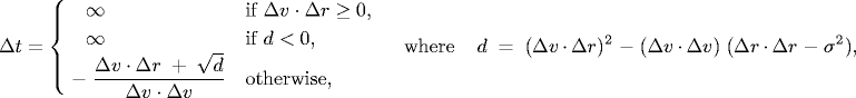
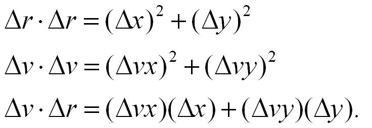
Substituting these four
equations into the previous one, solving the resulting
quadratic equation for Δt, selecting the
physically relevant root, and simplifying, we obtain an
expression for Δt in terms
of the known positions, velocities, and radii.
and
 EQUATION 3
 EQUATION 4
and
If either (Δv ⋅ Δr) ≥ 0 or d < 0, then the
quadratic equation has no solution for Δt
> 0; otherwise we are
guaranteed that Δt
≥ 0.
In the event the particles i and j will collide at the future
time we then need to determine the new positions and
velocities. There are three equations governing the elastic
collision between a pair of hard discs: (i)
conservation of linear momentum, (ii) conservation of kinetic
energy, and (iii) upon collision, the
normal force acts perpendicular to the surface at the
collision point. Students inclined towards Physics are
encouraged to derive the equations from first principles; the
rest of you may keep reading.
I) Collision between
particle and a wall:
When two hard discs collide,
the normal force acts along the line connecting their centers
(assuming no friction or spin). The impulse (Jx, Jy)
due to the normal force in the x and y directions of a
perfectly elastic collision at the moment of contact are:
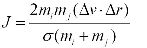
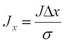 EQUATION 5
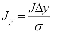 EQUATION 6
and where mi
and mj
are the masses of particles i and j, and σ, Δx, Δy
and Δ v ⋅ Δr are defined as above. Once we
know the impulse, we can apply Newton's second law (in
momentum form) to compute the velocities immediately after the
collision.
vxi' = vxi
+ Jx
/ mi, vxj'
= vxj - Jx
/ mj EQUATION 7
vyi' = vyi + Jy
/ mi, vyj'
= vyj - Jy
/ mj EQUATION 8
4)
Implementation
Download ALL of the following files:
main.m
start_position1.m
start_position2.m
create_event.m
update.m
box.m
plotbox.m
plotp.m
demo.p
Your
programming in this MP will involve completing the update
function.
We have given you the code
for the main function but it’s a good idea to look at the
code before you begin coding for the update function.
There is NO checker for this MP. So you must first
complete your code for the update function and then type
the following at the Matlab
prompt:
>> position
= main(500, 1.0e-11, 'start_position1');
or
>> position
= main(500, 2.0e-10, 'start_position2');
Your results should look similar to,
>> position
= demo(500,2.0e-10, 'start_position2');
You can type Control-C to terminate
execution.
4.1) The
main function a Step - by - Step Algorithm
1. The function ‘main.m’ which has three inputs, the
number of molecules N, the total time ‘total_time’ and a function that computes the
initial position matrix.
2. You will be able to download
two functions that compute the initial position matrix one
is named start_position1.m and the other start_position2.m.
The main function calls the start_position1.m or
start_position2.m function that you pass to main as a
function argument. Note that the start position matrix
has the form:
[ x , y , vx , vy , radius , mass ] and has ‘N’ rows.
3. We first plot the position
matrix.
4. Assign time = 0
5. Call the create_event
function to create initial event matrix.
6. Loop while time < total_time
a. Call the update function to
find the time to the next collision dt, and update both the
position and event matrices.
b. Increase time by dt.
c. plot the position matrix
4.2) Event Driven
Simulation … update function
When we update the event
matrix we will,
1) 1) find the minimum
time-to-collision value in the event matrix
2) 2) if the above event
corresponds to a particle-to-particle collision then add these
to the update list. The update list contains the particle number
(integer) for those particles we need to update the event
matrix, that is, for these particles we need to find their next
collision and put that collision in the event matrix. If the
next collision is particle-wall then just add this particle to
the list.
3) 3) check whether there
are other particles in the event list that were to collide with
the particle(s) in the list above. These particles should also
be added to the list.
4) 4) update the position
matrix using the math below above
5) 5) reduce the time
(every row in the event matrix) by the minimum time-to-collision
found in 1)
6) 6) call the create_event function and update all
rows in the event matrix that are in
the list from steps 2) and 3)
You are required to complete the
following two tasks.
First Task: Completing the code for the
function “update.m”.
Replace all the blanks with your code.
Second Task: Using the start_position1
call main as shown below. The start_position1
function assigns all particles to have the
same magnitude for velocity in the position matrix. Remember
if the velocity of a particle is V = [Vx,
Vy] then the magnitude of the
velocity would be,

After you run the Matlab
command,
>> position
= main(500, 8.0e-11, 'start_position1'); % this may take
20-30 minutes and if you run it on a lab computer while and
not remotely it will take less time
create a vector named velocities that
contains only the magnitudes of the velocities of the
particles and then display the velocities in a histogram,
(see Maxwell/Boltzmann to get an approximate view what
your plot should look like. Your plot would look closer to the
one shown if you increased the value 8.0e-11)
>> hist(velocities,14)
In the figure window click File/Save As and save
this image as velocities.fig.
Submit the following files:
:
I) update.m
II) velocities.fig
When you submit your
solution you can leave either one of the three
choices listed above.
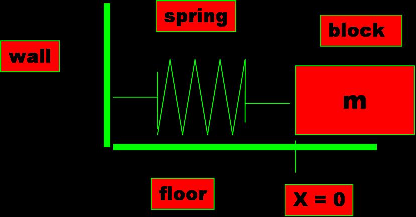
Assume that at t = 0 ,
x = 1 and v = 0. Use the time interval [0, 10].
3. Develop Algorithm (processing steps to solve
problem)
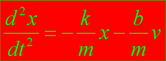
The ODE is described by the
harmonic oscillator:
% use m =
1 k = 100 b = 2 as values for now then after you have done a plot
then change b = 20 and later b = 5
5. Test and Debug the Code
Answer Part 3: Question 2
on your answer sheet.
6. Run the Code
After you have run the code,
plot the solution. Do this for each of the three cases for b =
2,20,5.
Answer Part 3: Question 3
on your answer sheet.