Particles and frictionless spheres are attractive components when simulating motion because their state does not include orientation or moments of rotation, only position and momentum.
1 Particle state and forces
Particle state is position, \mathbf{p}; particle velocity, which is the first derivative of position with respect to t and we’ll denote \.\mathbf{p}; and particle mass, m.
Physics notes various forces that apply to particles. Given a force \vec f, the corresponding acceleration is \"\mathbf{p} = \frac{1}{m}\vec f.
- Gravity
-
\vec f = G \dfrac{m_1 m_2}{r^2} in the direction of the other object. G = 6.6743×10^{-11} \frac{\text{m}^3}{\text{kg}\,\text{s}^2} is a universal constant.
For gravity caused by the earth near its surface, m_1 and r are constants and we have \vec f = g m where g = 9.80665 \frac{\text{m}}{\text{s}^2}.
For the acceleration caused by gravity near the earth’s surface we have \"\mathbf{p} = \frac{1}{m} g m = g.
- Drag
-
Assuming air is stationary and not rarified and that each particle is moving well below the speed of sound, draft force is linear if the speed is slow: \vec f = - c \vec v r^2 where c is a constant based on various characteristics of the air and the shape of the object; r is the radius of the particle; and \vec v is the velocity of the object. As the object speeds up this changes to a quadratic form \vec f = - c \vec v \|\vec v\| r^2.
The change happens smoothly between Reynolds Number 300 and 2000, where the Reynolds number for a sphere with radius r in room-temperature air is roughly 135{,}000\frac{\text{s}}{\text{m}^2} \|\vec v\| r. It is common to ignore this transition and just assume either that all particles are fast or all are slow.
- Collision
-
Collisions can be treated as instantaneous changes to a system that preserves total momentum and preserves or reduces total kinetic energy. That change in kinetic energy is determined by the elasticity of the collision.
When particles collide, only the speed in the direction of collision is impacted. When hitting a wall, that direction will be the surface normal of the wall. When hitting another particle, that direction will be along the line between the two particles.
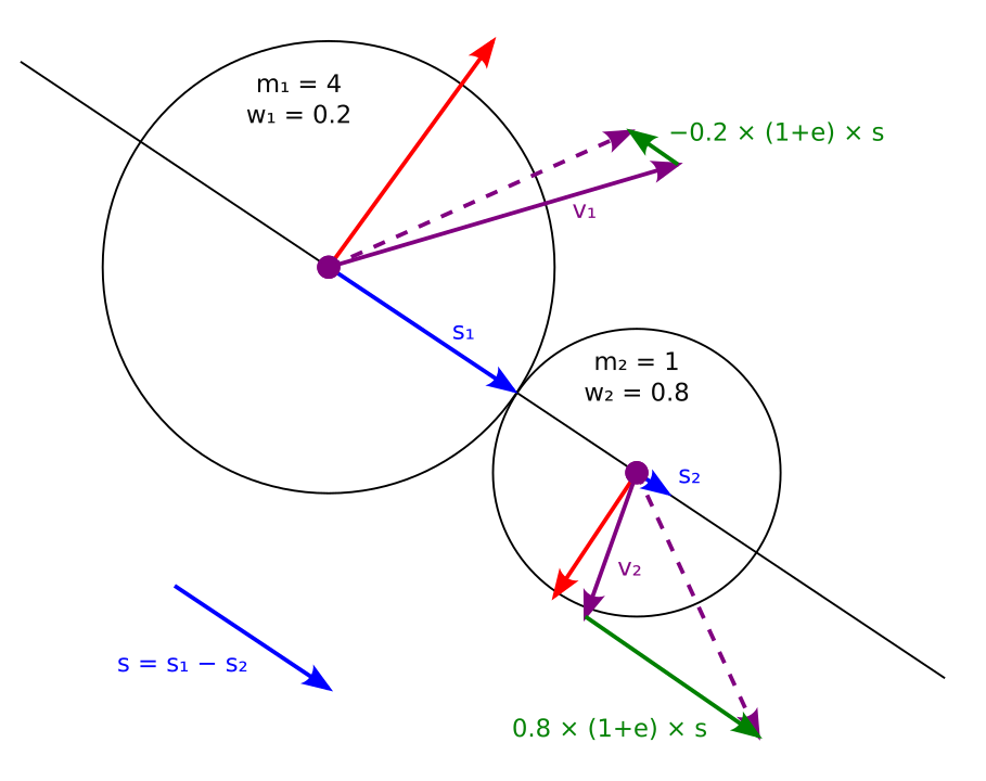
Illustration of collision handling The portion of velocity that is in the direction being changed is updated as follows:
A particle moves more if it contributes a smaller potion of the overall mass in the colliding system. We can quantify that as a
weight
between 0 and 1: w_i = \frac{m_j}{m_i+m_j}.Note that if either object is immovable we can use \displaystyle \lim_{m_i \rightarrow \infty} to get w_i = 0 and w_j = 1.
Let \vec d be a unit vector representing the collision direction
Let s_i be \vec v_i \cdot \vec d, the speed of particle i in the collision direction; and s be s_i - s_j, the net collision speed.
Add speed to resolve the collision; this fixing factor is \pm w_i (1+e) s \vec d where 0 \le e \le 1 is the elasticity of the collision.
2 Euler’s Method
The correct equation of motion is \mathbf{p}(t) = \mathbf{p}_0 + \.\mathbf{p}(t)t + \frac{1}{2}\"\mathbf{p}(t)t^2 but that’s usually not practical to compute because many of the terms depend on one another.
Euler’s method is a simple approximation that says
- \mathbf{p}_{\text{new}} = \mathbf{p}_{\text{old}} + \.\mathbf{p}_{\text{old}} \Delta t
- \.\mathbf{p}_{\text{new}} = \.\mathbf{p}_{\text{old}} + \"\mathbf{p}_{\text{old}} \Delta t
This accumulates error over time, roughly at O(t \Delta t). Because of the \Delta t term, it gives much better accuracy if the step size is small.
3 Runge-Kutta Methods
The correct equation of motion is \mathbf{p}(t) = \mathbf{p}_0 + \.\mathbf{p}(t)t + \frac{1}{2}\"\mathbf{p}(t)t^2 but that’s usually not practical to compute because many of the terms depend on one another.
The Runge-Kutta methods reduce the error of Euler’s method by taking multiple samples. There are many such methods; all share the basic idea that we can use an Euler timestep to estimate something about the function, but instead of updating the function based on that estimate we instead use it to make a better estimate.
The most common Runge-Kutta method is RK4, which runs as follows:
- Find what Euler would do
- And what Euler would do with half the timestep
- And what Euler would do with half the timestep if it used the \.\mathbf{p}_{\text{new}} from step 2 as its \.{\mathbf{p}}_{\text{old}}
- And what Euler would do if it used the \.{\mathbf{p}}_{\text{new}} from step 3 as its \.{\mathbf{p}}_{\text{old}}
- And average those four together, giving steps 2 and 3 twice the weight of steps 1 and 4.
This accumulates error over time, roughly at O(t \Delta t^4). The quartic power on \Delta t means it accumulates error very slowly for any reasonably-small \Delta t.
Runge-Kutta methods are rarely used in computer graphics. Generally we prefer to use the extra time RK4 needs on higher-resolution simulations instead of more accurate ones.
4 Position Based Dynamics
Position-based dynamics (PBD) stores only position, not velocity. It makes this seem physically realistic by using what the various physical laws will do to positions if integrated over a time step.
Let \mathbf{p}_i be the position at time step i and \Delta t_{i} be the time step between \mathbf{p}_i and \mathbf{p}_{i+1}.
If needed, the current velocity can be computed as \vec v_i = \dfrac{\mathbf{p}_{i} - \mathbf{p}_{i-1}}{\Delta t_{i-1}}. This comes directly from the definition of velocity as the change in position divided by the change in time.
Momentum adds \Delta t_i \vec v_i to the current position.
An accelerative force \vec f adds \frac{1}{2} \vec f \Delta t_i^2 to the current position.
Note that for simple forces like gravity this is just a constant vector addition each frame. The cumulative acceleration emerges from the combination of this addition and momentum.
Position based dynamics is simple and versatile, with a similar error accumulation as Euler’ method. It also has a similar space requirement as Euler’s method: Euler stores position and velocity per particle, PBD stores current and past position instead.
PBD works well when forces are applied more-or-less continuously, as with the interior of squishy and stretchy things. It does not handle the near-instantaneous impulses caused by the collision of rigid bodies well at all. Because it does not track velocity or kinetic energy, too-large timesteps cannot cause those values to explode as they can in some other approaches; however, conserving energy in PBD is also quite challenging.