Table of Contents
You will submit a webpage that has
- One canvas
- A set of controls to decide what geometry to generate
- A lit rendering of the generated geometry
As with the WebGL warmup, you’ll submit
an HTML file and any number of js, glsl, and json files. No image files
are permitted for this assignment. Also submit a file named
implemented.txt listing any optional parts you believe you
completed.
As with most assignments, this is divided into required and optional parts. For full credit, you need all the required parts of each assignment and an accumulated average of 50 optional points per assignment. Excess optional points at the end of the semester award extra credit, as explained in the grading policies.
This assignment, like all other assignments, is governed by the common components of MPs.
1 Starter templates
To provide consistency in user interface and page layout, we provide two files you should start from:
HTML File which as two
scriptelements you should edit, identified with comments in the file.Supporting JavaScript file which handles the option selection user interface. It shouldn’t require any editing; you don’t even have to look at it unless you’re curious.
scene-option-tree.jshad an error in the checkbox handling that was fixed 2023-03-29 11:12 CDT; if you use checkboxes and downloaded it before then, please re-download it now.
You are also welcome to use the matrix code we used in lecture if you would like. You may also use another JavaScript matrix and vector library, or write your own matrix code. You must not use third-party libraries other than for matrix and vector math.
The user interface in the starter files works as follows:
On the left are one or more radio buttons for types of geometry to
generate. Each one may have its own set of sub-options beneath it. Once
you’ve selected the options you want, pressing the button calls setupScene(scene, options)
where scene is the geometry type chosen and
options is a map of selected options for that geometry
type.
The set of options available is controlled by the global
controlOptions variable.
An example of using controlOptions
If we had
var controlOptions =
  {"terrain":
    {"label":"Required: Terrain"
    ,"options":
      {"resolution":{"type":"number","default":100,"label":"Grid size"}
      ,"slices":{"type":"number","default":100,"label":"Fractures"}
      ,"smooth":{"type":"checkbox","default":true,"label":"Smooth shading"}
      ,"erode":
        {"type":"radio"
        ,"options":
          {"rough":"No Weathering"
          ,"spheroid":"Spheroidal Weathering"
          ,"drain":"Hydraulic drainage"
          }
        }
      }
    }
  ,"torus":
    {"label":"Optional: Torus objects"
    ,"options":
      {"r1":{"type":"number","default":1,"label":"Major radius"}
      ,"r2":{"type":"number","default":0.25,"label":"Minor radius"}
      ,"res1":{"type":"number","default":48,"label":"Number of rings"}
      ,"res2":{"type":"number","default":24,"label":"Points per ring"}
      }
    }
  }
then there would be three radio buttons, each with different options:
|
Required: Terrain
Optional: Torus objects
Grid
size
Fractures
Smooth
shading
No
Weathering
Spheroidal
Weathering
Hydraulic
drainage
|
Required: Terrain
Optional: Torus objects
Major
radius
Minor
radius
Number
of rings
Points
per ring
|
setupScene("terrain", {"resolution":100, "slices":100, "smooth":true, "erode":"rough"})
|
setupScene("torus", {"r1":1, "r2":0.25, "res1":48, "res2":24})
|
2 Required (50 points)
You probably want to start using a simple fixed geometry object and get the view and lighting working, then start working on the terrain. Trying to get the terrain working before you can visualize it is generally a bad idea. You might find the lighting code from lecture particularly helpful in getting things set up.
- Button works
-
Each press of the button should
- clear any existing geometry
- generate new geometry based on the selected options
- display the geometry so created
- Geometry view
-
Geometry should be viewed
- in perspective
- with a moving camera
- from slightly above the geometry
- from a reasonable distance and zoom (most of the geometry should be on-screen, most of the view should be showing geometry)
Tip on fit and zoom
Using a view matrix is your best bet. That takes one input that’s the center of your view – put it in the center of your mesh. The camera position should be around 2 or 3 terrain diameteters away from the center horizontally and roughly half that far away vertically. - Lighting
-
You should have at least one sun-like light source and implement at least Lambert’s-law diffuse lighting; additional light sources and lighting models are available for optional credit.
If you get a speckled terrain, half colored and half black…
…then you probably (a) used triangle normals to compute vertex normals and (b) in each quad wound one triangle clockwise and the other counter-clockwise resulting in normals pointing both up and down. Fixing the winding or switching to edge-based normal computation should fix it. - Terrain
-
There must be a working option that generates a patch of fractal terrain using the Faulting Method. See also our description of the faulting method.
The grid dimension and number of faults should be user-selectable options. Your code must be able to handle any square resolution between 2×2 and 250×250. Regardless of the number of faults (as long as it is at least 1), the vertical separation from highest to lowest point should be between ½ and ¼ times as large as the horizontal separation of points on opposite sides of the grid.
Tip on vertical separation
The easiest way to control vertical separation is as a post-processing step:
- generate your geometry
- loop over all vertices, keeping track of the minimum and maximum x and z
- let h = (x_{\text{max}} - x_{\text{min}}) c where c is a constant between ½ and ¼ that you pick.
- if h \ne 0 loop over all vertices, replacing each z with \dfrac{z - z_{\text{min}}}{z_{\text{max}} - z_{\text{min}}}h - \frac{h}{2}
3 Optional
These are presented in roughly difficulty-per-point order, at least as I found them when implementing them to verify they were doable.
- Shiny (10 points)
- Implement a specular lighting component, using any standard specular lighting model. Regardless of the diffuse color of the object, the specular highlights should be the same color as the light (typically white).
- Height-based color ramp (20 points)
- Pick the (pre-lit) color of each fragment based on it’s world-space height so that the lowest areas are one color, the highest another, moving smoothly through other colors in between. Do this in the fragment shader with more than two colors: a rainbow, a heat map, etc.
- Rocky cliffs (20 points)
-
Anywhere the slope is steeper than some cut-off you pick, simulate the inability of soil and vegetation to cling to vertical surfaces by changing to a completely different material. Do this in the fragment shader with crisp cut-offs: each fragment is either cliff or not cliff, never half-way in between.
If you implement
Shiny
, also make the cliffs have a different size and strength of shininess than the shallower land. - UV-sphere (10 points)
-
Have an geometry option that makes a sphere instead of a terrain. Position the vertices so that edges form latitude and longitude lines around the sphere. Show the user two numeric options for the UV-sphere:
- Number of latitude rings, and integer ≥ 3. Include the two poles as two of these, so that 3 latitude rings has just the equator and the poles.
- Number of longitude slices, an integer ≥ 3. These each go from pole to pole on one side of the sphere only, so 3 longitude slices means the equator is a triangle.
As a simple check, if you use 3 latitude rings and 4 longitude slices, you should get the Platonic solid called an
octahedron.
You should be able to compute the surface normals exactly: the surface normal of a point on a sphere points directly away from the center of that sphere. For a unit-radius sphere centered at the origin, that means that \vec n = \mathbf{p}. If you don’t compute them exactly, make sure you don’t have any creases or seams, especially near the poles.
A UV-sphere with r rings and s slices should have no more than (r+1)(s+1) vertices, and if coded efficiently has only 2+(r-2)(s) vertices.
- Torus (15 points)
-
A torus is a tube with a circular cross-section looped into a circle. Doughnuts, bagels, O-rings, and inner tubes are all approximately torus-shaped.
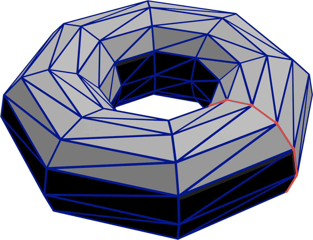
Have an geometry option that makes a torus instead of a terrain. Show the user three or four numeric options for the torus:
- Number of rings, and integer ≥ 3. See the above image for what a
ring
is. - Points per ring, an integer ≥ 3.
- Some way of controlling how
puffy
the ring is, from bagel (very puffy) to bicycle inner tube (not very puffy). This could for example be an inner and outer radius, a major and minor radius, a relative hole size, etc.
You should be able to compute the surface normals exactly: the surface normal of a point on a ring points directly away from the center of that ring. If you don’t compute them exactly, make sure you don’t have any creases or seams, especially where the mesh wraps.
A torus with r rings and p points per ring should have no more than (r+1)(p+1) vertices, and if coded efficiently has only (r)(p) vertices.
- Number of rings, and integer ≥ 3. See the above image for what a
- Spheroidal Weathering (20 points)
-
Add a numeric option to the terrain that controls the amount of spheroidal weathering to apply.
Spheroidal weathering is a phenomenon caused by heat, wind, and other generalized erosive forces and tends to erode sharp points much faster than it does flatter or concave areas.
A simple way to emulate this is to move each vertex part-way towards the average of its neighbors, iterating several times for more weathering. More accurate models compute curvature at a vertex1 and use that to determine offsets.
Make sure you move vertices in two passes: if you move vertex X and then update vertex Y based on X’s new position (instead of its old position) you’ll get unwanted biasing and sloping artifacts.
- Hydraulic erosion (30 points)
-
Implement hydraulic erosion, either grid-based or particle-based.
Let the user pick at least one numeric option controlling how many iterations the erosion is computed for. Hydraulic erosion also has several additional parameters (erosion rates, deposition constants, etc) you may either fix in your code or let the user specify, whichever you prefer.
- Icosphere (30 points)
-
Have an geometry option that makes a sphere instead of a terrain. Position the vertices by
- starting with the 12 vertices and 20 triangles of an icosahedron2
- repeating n times
- add a vertex in the center of each edge
- move the new vertices away from the center of the sphere to be the same distance from the center as the original vertices are
- connect the new vertices to the old to make 4 triangles out of each previous triangle
n \ge 0 should be a numeric option shown to the user for the icosphere. Only test your code with fairly small n; by n=8 there will be over 1 million triangles, enough to overtax some GPUs.
An icosphere with n levels of subdivision has exactly 10(4^n)+2 vertices.