Recursion

Algorithms

So far, we’ve looked at a few models of computation, formal descriptions of how computation can be done, and we focused exclusively on models for generating or recognizing strings in a particular language. We mostly looked into what is possible with our models while not worrying too much about what can be done efficiently. For example, we didn’t care about how many states an automaton had. The important thing was whether an automaton existed at all for a given language, and all else being equal, having one that could be understood by ourselves and others was the important thing.

For the next several weeks, we’re going begin focusing on how efficiently we can accomplish certain tasks by designing efficient algorithms. Correctness will still be our primary concern, but we’re also going to try to make them run quickly, and occasionally (if we do so at all) we’ll discuss how much space they require.

Because we’re now dealing with more practical concerns, we are going to use a more practical models of computation. We’ll typically be using what is often called the Real RAM model. It’s not worth going into exact specifics, the model lets you do pretty much anything you’d expect from a modern programming language like C++ or Python. In more detail than I’ll probably say out loud in lecture:

• We can store arbitrarily large real numbers in constant sized units of memory and access them in constant time.
• We can do basic arithmetic operations like addition, subtraction, multiplication, division, floors, ceilings, (and maybe square roots?) between a constant number of operands in constant time each.
• We have arrays where the member at a given index can be read or written to in constant time. I’ll typically denote them as A[i~..~j] where i and j are the least and highest valid index. We read or write individual elements A[k].
• We can store and follow individual pointers or references in constant time.
• We can do function calls in constant time each (and passing in a (sub)array takes no additional time; you can think of doing so by reference.)
• We while and for loops as well.

Occasionally (including during the next lecture,) we’ll use other models, and we’ll make it clear when we’re doing so.

“Describing an algorithm”

Please look over Homework Policies page again for details on what we mean when we ask you to “describe an algorithm”.

In particular, we are not asking for code. We are not compilers, and your graders cannot be expected to read perl, or Rust, or even Python. You may choose to use pseudocode, and it is probably the easiest way to describe the kinds of algorithms we’ll be discussing this week. However, plain English should be enough to describe every algorithm you design. The general rule is that a competent programmer should be able to implement your algorithm in their favorite language using a software library containing everything we’ve seen in 225 and in this class, without having to ask for more details or understanding why your algorithm is correct.

Every algorithm description needs to include a worst case¹ run time analysis using asymptotic (big-Oh) notation. It’s often enough just to point out how much nesting occurs with some loops, e.g., “It’s a doubly nested for loop over n elements so O(n^2),” but you may (especially this week) need to set up and solve a run time recurrence. We’ll review how to do so.

We likely won’t tell you what run time bound we’re expecting to see. Doing so tends to lead to many incorrect algorithms that match the bound we ask for which is always worse than a correct algorithm that happens to be slower. Assuming a correct algorithm description with unexpected run time, we’ll give partial or even extra credit depending on how much slower or faster it is compared to what we expect.

Finally, we’d like to know why your algorithm is correct. For solutions based on the basic paradigms we cover in class, you won’t need to say anything more than what is mentioned in the standard rubrics. They’re designed to make it clear what your algorithm is doing while also making it clear why it works. However, if you do anything outside these basic paradigms, then you’ll likely need to say more. In particular greedy algorithms will always require a formal proof of correctness, because it is very easy to describe incorrect greedy algorithms, and we have to assume that’s what you’ve done until you prove otherwise.

Alright, let’s actually get to it.

Recursion

The most powerful tool we have for designing efficient algorithms is reductions, solving some problem A using an algorithm for a problem B without relying on understanding of how the algorithm for B works. In fact, we’ll be relying heavily on reductions for the rest of the semester, although not necessarily always to show existence of fast algorithms.

There’s a particular kind of reduction that we’re going to lean on heavily for the next three weeks (and occasionally afterward up to the next midterm,) and we’ve already seen it in a sense. When we wanted to prove things about strings, we took a claim and reduced the proof to the same claim but with smaller associated numbers. Then, the Induction Fairy would promise us the “smaller” claim is correct and let us finish our case analysis. We’re going to do the exact same thing with algorithms, except now most people call the process recursion.

Recursion is reducing a problem A to smaller instances of the same problem A. The reason it works just another example of induction. If we can reduce our given problem (say, of size n) to a smaller instance (say, of size k < n), we may assume the Recursion Fairy will correctly solve it for us. How the Recursion Fairy solves the problem isn’t our concern, and not having to worry about it frees up our brains to do other things, like figure out how to make smaller instances of the problem for the Recursion Fairy to solve. In instances where we can’t reduce to a smaller instance (the base cases,) we can’t call upon the Recursion Fairy. However, we should be able to solve the base cases by some simple brute force method.

Example: Tower of Hanoi

Sorry, that’s a lot of lofty high level concepts, so let’s relax with a puzzle. In 1883, Édouard Lucas created a puzzle based on a stack of disks sitting on one of three pegs. This puzzle is called the Tower of Hanoi. Here are the rules for the puzzle:

• There are three pegs upon which we may place stacks of disks.
• Initially, all the disks are stacked on peg in decreasing order of size from bottom to top.
• In each step, you may move the topmost disk off one stack of disks to another disk.
• You may never place a larger disk on top of a smaller one.
• The goal is to move all disks from the starting peg to a different peg.

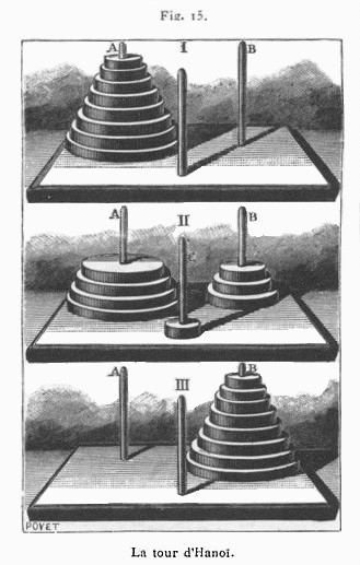
This puzzle looks complicated! But maybe we can use this lecture’s subject of recursion to get a handle on it. If we can somehow reduce a given instance of Tower of Hanoi to a smaller instance of Tower of Hanoi, we might succeed.

Let’s say disks are numbered 1 to n in increasing order of size and we want to move all of them from peg A to peg B (and there’s a peg C, also.) If we can reduce solving the puzzle to moving around one or more smaller sets of disks that abide by the exact rules of the same puzzle, we might be able to succeed.

Fortunately, we can do exactly that. The first (smaller) n - 1 disks don’t have their movement affected by disk n at all, because it is bigger than all of them. We can treat those n - 1 disks exactly the same as an (n-1)-disk instance of our problem. Incidentally, the only thing we can do with disk n is move it from its otherwise empty peg to another empty peg, and only after the disks on top have been removed first. Therefore, to move disk n from peg A to peg B, we have to first move the smaller n - 1 disks to peg C (using recursion). Then, we can move disk n to peg B. Finally, we can complete the puzzle by moving the n-1 smaller disks from peg C to lie on top of disk n on peg B.

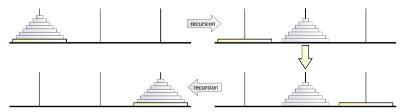
Should we need to worry about how to move the smaller stack of n - 1 disks? NO! The Recursion Fairy is very insistent that it’s not our concern.

The only situation in which we can’t move the smaller n -1 disks is when n = 0, implying n - 1 is negative. Fortunately, there’s nothing to do in that case.

More succinctly, suppose we want to move n disks from peg src to peg dst using peg tmp as temporary storage for the disks. We could describe the process using pseudocode as follows:

We just described an algorithm to solve the Tower of Hanoi puzzle! If this were a homework or exams problem, we’d still need to figure out the “running time” of the algorithm to get full credit. In this case, the running time is best expressed as the number of moves as a function of n. Specifically, let T(n) be the number of moves to solve n-disk Tower of Hanoi. We just discussed a recursive algorithm, which means its running time is based on the running time of its two recursive calls. In other words, T(n) can be written as a recurrence, and if we solve the recurrence, we get our answer. T(n) = \begin{cases} 0 & \text{if $n = 0$}\\ 2T(n - 1) + 1 & \text{otherwise}. \end{cases}

You may not have seen how to solve a recurrence of that form, but maybe we can guess the solution by looking at some small values of n:

n	0	1	2	3	4	5
T(n)	0	1	3	7	15	31

Guess: T(n) = 2^n - 1.

While we will be using it implicitly through recursion, that might be the last formal induction proof we see for the semester.

Example: Mergesort

Let’s look at another example that feels a bit more “computery”. Given an array A[1~..~n] of say, real numbers, we want to rearrange them so that A now contains them in sorted order. One method of doing so was developed by von Neumann in 1945: mergesort.

1. Divide the array into two disjoint subarrays of roughly equal size.
2. Recursively sort each of the two subarrays.
3. Merge the two newly sorted subarrays into one big sorted array.

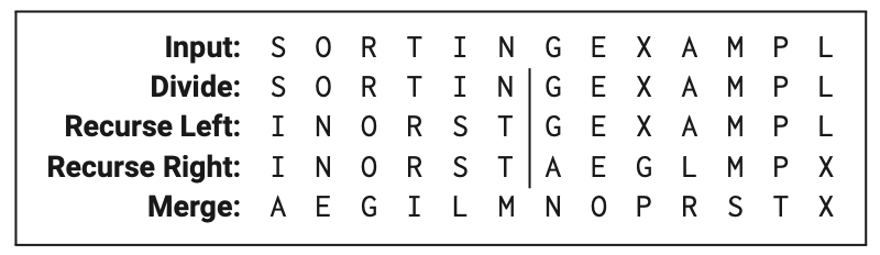
The only time this strategy fails to produce two strictly smaller arrays upon which we can recurse is when n \leq 1, but there’s nothing we need to do in that situation anyway.

Here’s a pseudocode description: \text{MergeSort}(A[1~..~n]) sorts the array A in place. It makes a call to a subroutine \text{Merge}(A[1~..~n], m) that sorts A assuming A[1~..~m] and A[m+1~..~n] are already sorted.

But how do we perform the merge?

Think recursively!

The first element of sorted A is the smallest element of either A[1~..~m] or A[m+1~..~n], and that smallest element must appear in the first position of its subarray. So, we take the smaller of the two first subarray elements. Now we have all of the subarray we didn’t pull from left to merge and the rest of the one we did. The two subsubarrays are still sorted, though, so we can recurse! If we faithfully follow this train of thought and trust the Recursive Merge Fairy, then we can implement Merge as an explicit recursive procedure. However, \text{Merge} is typically written with a for loop (yawn.)

A full formal proof of correctness would use induction. Once to prove that Merge is correct and then again to prove that MergeSort is correct assuming Merge is correct. The details are in Jeff’s book.

However, we don’t expect you to give formal proofs of correctness for basic recursive algorithms. The important thing here is that we carefully defined what the MergeSort and Merge procedures do with their inputs and wrote them in a clear way. If somebody else really wanted to do the proof, they probably could.

We do need to figure out the running time, though. Merge just uses a pair of for loops over n values with constant work in each iteration, so it runs in O(n) time. For the main procedure, let T(n) be the worst-case running time of MergeSort over an n-element array. Based on the size of the two recursive calls, we get T(n) = T(\lfloor n / 2 \rfloor) + T(\lceil n / 2 \rceil) + O(n) with T(n) = O(1) for all n = O(1).

So, now we just need an asymptotic (i.e. big-Oh) bound on T(n). But how do we get one?

First, dividing the subproblem sizes by a constant has a much bigger effect on the final asymptotic growth of T(n) than the floor and ceiling do, so we can safely ignore them and solve T(n) = 2T(n / 2) + O(n) instead. If you’re interested, Erickson’s Algorithms book has details on precisely why it’s OK to do so.

With that done, it’s possible you’ve seen a some kind of method or theorem for handling this style of recurrence in another class. It might serve us well in this case, but it won’t last even as far as the next lecture. Besides, we don’t want to be slave or even apprentice to a theorem. What we will do instead is tackle the analysis more directly by using a recursion tree; it’s how we’d prove that theorem (which I’ll now never bring up again), anyway.

A recursion tree is a rooted tree where every node represents is a recursive subproblem encountered while running the algorithm on a particular problem instance. (I may refer to a subproblem and its node using the same notation.) For each direct recursive call v made by subproblem u, the node u has the node for v as one of its children.

The nodes may contain values based on the reason for considering the recursion tree. Right now, we want to analyze running time of an algorithm, so we’ll give each node a value equal to the time spent in that node’s subproblem not including time spent in that subproblem’s own recursive calls. Then, the sum of all node values will equal the total time spent running the entire algorithm. Finally, we’ll skip writing the big-Oh inside the nodes, because we’re only going for an answer that’s correct up to constant factors anyway. Doing so will actually help to make things more clear, because when we’re a few levels down the recursion stack, the constants will start to actually matter.

Here’s the recursion tree for mergesort on an array of size n:

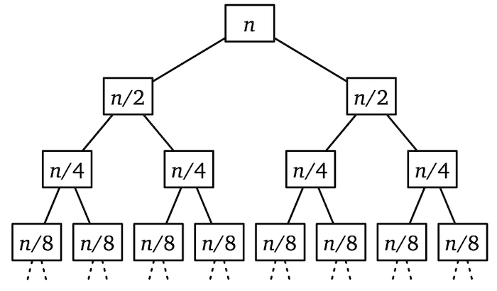
The running time of mergesort T(n) is the total time spent in all of its subproblems, so we need to sum up those node values. Typically, the easiest way to find this sum is to figure out the sum for each individual level and then to sum up all the levels. (Addition is associative.)

For mergesort, each level sums to be at most n. How many levels are there? We divide the problem size by 2 every time, so the depth of the tree is some k where n / 2^k = 1 (plus or minus 1), which occurs if and only if n = 2^k which occurs if and only if k = \log_2 n. In other words, we can only divide by 2 a total of \log_2 n times before hitting a the constant sized base case. So T(n) = O(n \log_2 n) = O(n \log n). Which you may have already known.

Example:: Quicksort

There’s another popular sorting algorithm known for its use of recursion: quicksort by Tony Hoare (’61). Here, we

1. Choose a pivot element from the array.
2. Partition the array into three disjoint subarrays that contain, in order, elements smaller than the pivot, the pivot itself, and elements larger than the pivot.
3. Recursively quicksort the first and last subarrays.

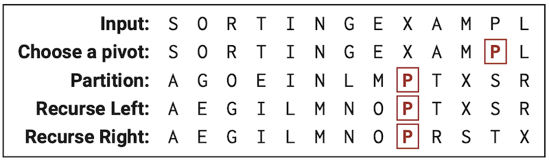
Here’s some pseudocode. \text{QuickSort}(A[1~..~n]) sorts A. It relies on a subroutine \text{Partition}(A[1~..~n], p) which partitions A around the pivot element located at index p (again, us writing A[1~..~n] means indexing starts at 1). This method of partitioning is attributed to Nico Lomuto.

Again, a formal proof of correctness would use induction both to prove correctness for \text{Partition} and for quicksort itself. The proof for \text{Partition} argues that at the end of each iteration of the main loop, everything in A[1~..~\ell] is less than A[n] and nothing in A[\ell+1~..~i] is less than A[n].

Now for running time. Just like \text{Merge}, \text{Partition} runs in O(n) time. However, the sizes of the two recursive calls are no longer fixed and instead depend upon the rank of the pivot element. An element in an array has rank r if it is the rth smallest element in the array. Since we’re sorting and using 1-indexing, the rank of the pivot is equal to its index after calling \text{Partition}.

Let T(n) be the worst case running time on an array of n elements (I’m using \Theta here, because I want to emphasize a tight asymptotic bound that applies from both above and below), and let r be the rank of the chosen pivot. T(n) = \Theta(n) + \max_{1 \leq r \leq n}\left(T(r-1) + T(n - r)\right).

Ideally, r would be really close to n/2 and we’d get two balanced subproblems like before, but there’s no guarantee that is the case. In particular, we could have r = 1 or r = n, giving us T(n) \geq \Omega(n) + T(0) + T(n - 1). As shown by the following recursion tree, that leads to a pretty bad run time!

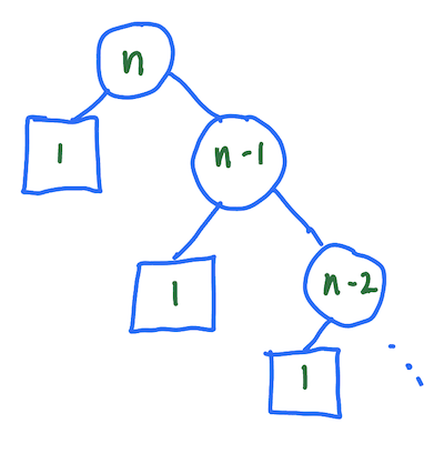
In this case of r being really big or really small, each level i sums to at most n - i + 1, and we keep going until level k where n - k = 1, meaning k = n - 1. We have T(n) \geq \Omega\left(\sum_{i = 0}^{n - 1} (n - i + 1)\right) = \Omega(n^2). Fortunately, each level is at most n + 1 no matter what choices of r we use, so we can also conclude T(n) = O(n^2). Quicksort always takes at most O(n^2) time, and it can take as long as \Omega(n^2) time, so the worst case running time is \Theta(n^2).

In general for this class, you won’t need to go out of your way to verify that your upper bound on the running time can actually be achieved. I’m just doing it here to show that, no really, quicksort is worse than you might think in some cases. In fact, you can even describe instances for all n for which most popular pivot selection heuristics like median-of-three will still give you \Theta(n^2) running time.

So is there a way to quickly choose a pivot that lies near the middle of the sorted array? We’ll see in the next lecture.

Divide-and-conquer

Both mergesort and quicksort are examples of divide-and-conquer algorithms:

1. Divide the given instance into several independent smaller instances of the same problem.
2. Delegate each smaller instance to the Recursion Fairy.
3. Combine the solutions of the smaller instances to make the solution to the given instance.

Typically, each recursive instance is a constant factor smaller than the input instance, and you can use recursion trees to figure out the running time. The smaller instances don’t necessarily have to partition the original instance like we saw in these two examples. We’ll see two examples of more surprising divide-and-conquer algorithms in the next lecture.