(Karp) Reductions
Motivation
The last several lectures have been about the design of efficient algorithms: you’re given a problem you want to solve, and if you’re fortunate, you can apply something like divide-and-conquer, dynamic programming, or a graph reduction to make an algorithm that solves that problem efficiently. Now it’s time to flip things around by asking when we aren’t so lucky. We’ll be discussing ways to argue that certain problems cannot be solved efficiently. In some cases, that means a problem has no “efficient” solution for a given definition of efficiency. In other cases, it means no algorithm exists at all to solve the problem in a finite amount of time!
These kinds of arguments and the established theory around them require a level of precision that’s a bit higher than what we were using with algorithm design, especially when we start talking about whole complexity classes of problems defined based on how much time or other resources you need to solve them. We need to understand precisely the kinds of problems we’re dealing with. Eventually (but not quite yet), we’ll also have to review the precise model of computation we’re considering. So for this lecture, we’re going to go over the types of problems we’ll be dealing with and then (re-)introduce our most powerful tool for arguing certain things are hard.
Decision problems and languages
So far, we’ve mostly (but not entirely) focused on optimization problems: given an input, there are a set of feasible solutions each with their own value, and we want to compute the minimum or maximum value of these feasible solutions. For example: Given G = (V, E), s \in V, and t \in V, what is distance from s to t?
However, the theory around problem difficulty more typically addresses decision problems: given an input, decide Yes or No: does that input have the desired property you like.
These kinds of problems are more closely related than you might think: given an optimization problem P, I can define a decision version of P which takes the normal input of P and a parameter k. We ask, is there a solution of value at most/at least k? For example: Given G = (V, E), s \in V, t \in V, and an integer k, is there a path from s to t with at most k edges?
It works the other way as well. We can typically solve an optimization problem by doing repeated calls to the corresponding decision problem. In this example, we do a binary search for the smallest k for which the answer is Yes. You’ll get to practice doing designing these sorts of optimization algorithms in the next lab.
So why do we focus on decision problems? It turns out decision problems are just another way of describing something we saw all the way back during the second lecture. Formally, whenever we talk about a fixed problem’s input, what we’re really referring to is an arbitrary string x, typically over \{0, 1\}, that describes that input, and when we’re talking about a fixed decision problem, there is a subset of strings that describe Yes instances of that particular problem.
And we have a particular term for a subset of strings, language. Every decision problem A has an associated language L_A of those strings that are Yes instances of A. The opposite is true as well. For any fixed language L, we can define the problem of deciding if a given string belongs to L. These two concepts of decision problem and language are so closely entwined that I may use them as synonyms or talk about a language like SHORTESTPATH instead of L_{\text{SHORTESTPATH}}. I’ll try to keep the notation consistent, though, but I’m sure I’ll slip up especially in the last week of class when languages take priority.
Reductions between decision problems
Right then, so let’s suppose I have a decision problem A and we want to know if there is an efficient algorithm for A. Unfortunately, we don’t have great tools for definitively answering that question, assuming A has an algorithm at all. But what we can do is compare difficulty between pairs of problems. And the way we do so is by applying a technique we used over and over and over again while designing algorithms, a reduction.
We reduced several optimization problems to solving a problem in a graph. For dynamic programming, we reduced a function evaluation to a “smaller” evaluation of the same problem. Recursion is, by definition, the reduction of a problem to a smaller version of that same problem.
The same principle applies for what we’re doing to study how difficult certain problems are to solve, except we can often restrict the kinds of reductions we need to use for decision problems.
A many-one reduction from a decision problem A to a decision problem B is a computable function f such that x is a Yes instance of A if and only if f(x) is a Yes instance of B, i.e., x \in L_A if and only if f(x) \in L_B. Here, computable means there’s an algorithm for f, but we don’t care about its running time. The existence of f suggests an algorithm for A; given input x, apply f to x and return the answer to f(x) on B.
There’s a particular kind of many-one reduction that is especially interesting to us, though, especially for the next few lectures. In a polynomial time many-one reduction or Karp reduction from A to B, the function f applied to input x can be computed in O(\text{poly}(|x|) time. If one exists, we write A \leq_P B. Thanks to the equivalence of decisions problems and languages, we might also write L_A \leq_P L_B.
But why is polynomial time? It composes well.
Lemma: If A \leq_P B, and B has a polynomial time algorithm, then A has a polynomial time algorithm.
Proof: Suppose we can reduce A to B using function f, function f takes O(|x|^c) time on input x, and B has an algorithm that takes O(|y|^d) time on an input y. Then, |f(x)| \leq |x|^c, and we can solve A in O(|x|^c + (|x|^c)^d) = O(|x|^{cd}) time.
The contrapositive of the above lemma is what we really care about for these next couple lectures.
Corollary: If A \leq_P B, and A has no polynomial time algorithm, then B has no polynomial time algorithm.
Examples: Independent set and friends
We’ll start by considering the following three decision problems. All three take an undirected graph G = (V, E) and an integer k as input.
- IndependentSet (IS): An independent set is a subset of vertices with no edges in between them. We want to know if there is an independent set of size k.
- Clique: A clique is a complete subgraph; there is an edge between every pair of its vertices. We want to know if there is a clique of size k.
- VertexCover (VC)): A vertex cover is a subset of vertices where every edge in the graph is incident to at least one vertex. We want to know if there is a vertex cover of size k.
From left to right below, we have an independent set, a clique, and a vertex cover, each of size 4.
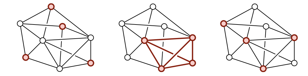
I don’t know of an efficient algorithm for any of these three problems, and by efficient, I mean the algorithm runs in some time polynomial in O(|V| + |E|). But what I do know is if we can find an efficient algorithm for any of them, then we have an efficient algorithm for all three. Equivalently, if there is no efficient algorithm for any one of them, there is no efficient algorithm for any of them.
Let’s say we want to solve IndependentSet. We’re given our graph G = (V, E) along with an integer k. We’re going to do a polynomial-time many-one reduction to Clique. Specifically, we construct an instance (\overline{G} = (\overline{V}, \overline{E}), k') of Clique where \overline{G} is the complement of G, and k' = k. In more detail.
- \overline{V} = V (it’s the same set of vertices),
- \overline{E} = \{uv \mid uv \notin E\},
Building the Clique instance takes polynomial time O(|V|^2).
These reductions tend to get fairly subtle, and much more so than the reductions to graph problems we did the last couple weeks, so we need to prove correctness. Specifically, we need to prove (G, k) is a Yes instance of Independent Set if and only if (\bar{G}, k') is a Yes instance of Clique.
Proof: Let S \subseteq V be an independent set of size k in G. For all u, v \in S, edge uv \notin E, so uv \in \bar{E}. Subset S is a clique of size k in \bar{G}.
Now, let S \subseteq V be a clique of size k in \bar{G}. For all u,v \in S, edge uv \in \bar{E}, so uv \notin E. Subset S is an independent set in G
We just proved the following theorem.
Theorem: \text{IS} \leq_P \text{Clique}.
In other words, Clique is at least as hard as IndependentSet up to polynomial terms and factors.
It’s important to recognize that we don’t need to know an efficient algorithm for Clique for this reduction to be correct. In fact, we just proved that no polynomial time algorithm for Clique exists if one does not exist for IndependentSet (we’ll get to why one may not exist for IndependentSet in the next lecture). The important thing is we transformed an instance of IndependentSet into an instance of Clique in polynomial time. It turns out the exact same reduction f shows \text{Clique} \leq_P \text{IS} as well, but that is rarely the case.
We can do a polynomial time reduction from IndependentSet to VertexCover, also. Here, we’re again given a graph G = (V, E) with |V| vertices and |E| edges along with an integer k as the input for IndependentSet. We now construct an instance (G' = (V', E'), k') of VertexCover where
- V' = V (it’s the same set of vertices),
- E' = E (in fact, it’s the same graph!),
- k' = n - k (but that integer parameter changed).
The reduction takes polynomial time O(1). (Or O(n) if you insist I make a new copy of the graph).
Now we need to prove (G, k) is a Yes instance of IndependentSet if and only if (G', k') is a Yes instance of VertexCover.
Proof: Let S \subseteq V be an independent set of size k in G. Now, let S' = V \setminus S. We have |S'| = n - k. Consider any edge uv \in E. It is not the case that both u and v are in S. Therefore, at least one of u or v is in S'. We include at least one vertex of every edge in S', so S' is a vertex cover.
Now, let S' \subseteq V be a vertex cover of size k' = n - k in G'. Let S = V \setminus S'. We have |S| = n - (n - k) = k. Consider any edge uv \in E. At least one of the u or v is in S'. Therefore, it is not the case that both u and v are in S. We never include both endpoints of an edge in S, so S is an independent set.
We just proved another theorem.
Theorem: \text{IS} \leq_P \text{VC}.
This reduction reverses easily as well, but again, that’s not typically the case.
If we’d like, we can chain the reductions shown above. Given an instance of Clique, we can reduce to VertexCover by first applying the reduction from Clique to IndependentSet and then applying the reduction from IndependentSet to VertexCover. Between composition and reversal of the reductions, it turns out all three problems are equally difficult up to polynomial overhead.
Theorem: Let A and B each be one of IndependentSet, Clique, or Vertex. Then, A \leq_P B.
Example: Directed and undirected Hamiltonian cycle
There likely won’t be time during in-person lecture, but lets look another collection of (two) problems. Given a graph, a Hamiltonian cycle is a cycle that includes every vertex exactly once. We have two decision problems this time:
- UndirHamCycle: Given an undirected graph G = (V, E), does it contain a Hamiltonian cycle?
- DirHamCycle: Given a directed graph G = (V, E), does it contains a Hamiltonian cycle?
This first theorem is maybe not too surprising.
Theorem: \text{UndirHamCycle} \leq_P \text{DirHamCycle}.
We need to describe a reduction to prove this theorem. Suppose we’re given an instance of UndirHamCycle, an undirected graph G = (V, E). We build an instance of DirHamCycle, a directed graph G' = (V', E') where
- V' = V (again, same set of vertices), and
- E' = \{u \to v \mid uv \in E\} (i.e., we include both orientations of every edge in G).
The reduction takes polynomial O(|V| + |E|) time.
Now we need to prove G has a Hamiltonian cycle if and only if G' has a Hamiltonian cycle.
Proof: Let C = \langle v_1, v_2, \dots v_{n-1}, v_1 \rangle be a Hamiltonian cycle in G. For each consecutive pair u, v in C, there is a directed edge u \to v in G'. Therefore, C is a Hamiltonian cycle in G' as well.
Let C = \langle v_1, v_2, \dots v_{n-1}, v_1 \rangle be a Hamiltonian cycle in G'. For each directed edge u \to v in G', there is an undirected edge uv in G. Therefore, C is a Hamiltonian cycle in G as well.
Done. But what about the other direction?
Theorem: \text{DirHamCycle} \leq_P \text{UndirHamCycle}.
We again need to describe a reduction. Suppose we’re given an instance of DirHamCycle, a directed graph G = (V, E). We build an instance of UndirHamCycle, an undirected graph G' = (V', E') where
- V' = \{v_- \mid v \in V\} \cup \{v_0 \mid v \in V\} \cup \{v_+ \mid v \in V\} (i.e., there are three distinct copies of each vertex), and
- E' = \{u_+ v_- \mid u \to v \in E\} \cup \{v_- v_0 \mid v \in V\} \cup \{v_0 v_+ \mid v \in V\}.

The reduction takes polynomial O(|V| + |E|) time.
The intuition here is that a cycle passing through directed edge u \to v in G can be represented by one going through u_- to u_0 to u_+ to v_- in that order in G'. Despite the mention of intuition, it’s still not obvious that our reduction actually works this time. We need to carefully show directed G has a Hamiltonian cycle if and only if undirected G' has a Hamiltonian cycle.
Proof: Let C = u \to v \to w \to \dots \to u be a Hamiltonian cycle in G. Let C' = u_- \to u_0 \to u_+ \to v_- \to v_0 \to v_+ \to w_-, \dots \to u_- in G'. Every edge used in C' exists in G'. Also, cycle C includes every vertex in G exactly once (not counting the return to u), so it goes through every triple of vertices in G' exactly once. Walk C' is a Hamiltonian cycle in G'.
Now, let C' be a Hamiltonian cycle in G'. Pick any u_0 visited by C'. It is only adjacent to u_- and u_+. Graph G' is undirected, so we can reverse C' if necessary to make it visit u_-, u_0, and u_+, in that order. Now consider any other w_0. By induction on the number of vertices between u_0 and w_0 in C', we may assume C' visits w’s collection of vertices by leaving some v’s collection from v_+. Then C' goes through v_+ w_- and then through w_-, w_0, and w_+ in that order. Therefore, C' has the form u_- \to u_0 \to u_+ \to v_- \to v_0 \to v_+ \to w_-, \dots \to u_-. Let C = u \to v \to w \to \dots \to u. By construction of G', each of the edges in C exist in G. Also, C' visits every vertex v_0 exactly once, so C visits every vertex v exactly once. Walk C is a Hamiltonian cycle in G.
Conclusion
We saw a couple polynomial time many-one reductions between samey looking problems. A polynomial time reduction from decision problem A to decision problem B tells us a couple things.
- If we ever find an efficient (polynomial time) algorithm for problem B, then we immediately know of one for problem A.
- In contrast, if there is no polynomial time algorithm for problem A, then there is no polynomial time algorithm for problem B.
So, let’s suppose there is some decision problem B for which we just cannot think of a polynomial time algorithm, and we believe no such thing exists. Are there any other decision problems A with no polynomial time algorithm that we can reduce to B?
The answer is a resounding kind of. I mean, we have pretty good reasons to believe we know of some, and that’s the subject for the next lecture.