Graphs

We’ve now had several lectures devoted using recursion to design algorithms for novel problems. The next few lectures are going to be a bit different. We’re going to be covering some specific algorithms for graphs that are interesting theoretically and have lots of applications within and outside of computer science. While I’ll still ask you to design a couple of algorithms for graphs using similar techniques to what I’ll show in lecture, I’ll also ask you to design algorithms for graphs and other settings that merely do reductions to the major algorithms I’m going to show.

Before getting into specifics, though, we need to review what a graph is and see how they’re typically represented on a computer or in an algorithm. A common way to imagine graphs is to think of those things you get from a planar drawing. Here are two different planar drawings of the same (disconnected) graph.

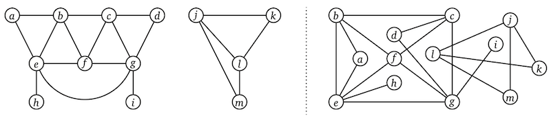
However, the actual definition of a graph is a bit more abstract than suggested by these drawings, and this abstraction is what makes graphs so helpful in designing algorithms for all sorts of problems. Formally, a graph G = (V, E) consists of a (non-empty) arbitrary finite set V of vertices (or nodes) and a set of pairs of elements of V denoted E and called the edges. Some graphs are undirected and others are directed.

• In an undirected graph, the pairs defining the edges are unordered. In this class, I’ll often write uv to denote an edge between vertices u and v even though the basic definition suggests it should be written \{u, v\}.
• In a directed graph, the pairs defining edges are ordered, and we’ll often write u \to v to denote what the definition suggests should be (u, v).

Again, these vertices themselves are arbitrary and that leads to elegant ways to model many different phenomena as graphs. One example is an intersection graph where the vertices are geometric objects, and the edges are pairs of objects that intersect.¹

Every instantiation of a recursive algorithm has a dependency graph where vertices are subproblems that are encountered while running the algorithm and there is an edge u \to v whenever subproblem u does a recursive call to subproblem v. For example, here is the dependency graph for computing the nth Fibonacci number recursively.

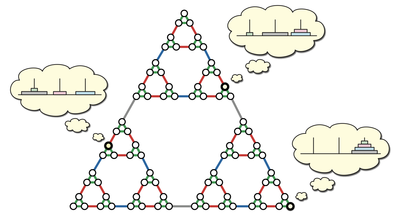
The configuration graph of a game, puzzle, etc. has a vertex for every distinct configuration the thing can take and a (possibly directed) edge between configurations that can be obtained consecutively. Here’s the configuration graph for the 4-disk Tower of Hanoi.

Finally, one last example that we’ve encountered many times throughout this class explicitly are the state-transition graphs for NFAs. The states of the NFA are vertices of the graph, and there are edges u \to v whenever you can transition from u to v by reading an input symbol.

One of your main challenges these next few weeks will be to recognize graphs in the problems we give you so can easily can solve the problem by calling the appropriate graph algorithm.

Data structures

But before we can see some graph algorithms, we need to discuss how a computer stores a graphs as a data structure so we know what kinds of basic operations we can perform on them and how quickly. Let G = (V, E) be a graph (directed or undirected). We’ll assume G is simple, there is at most one edge u \to v or uv for each pair (u, v) and no loops v \to v or vv. I’ll try to write |V| or |E| when counting vertices and edges or including those numbers in asymptotic bounds. However, I may sometimes accidentally use V or E as their cardinality like Erickson’s book does.

For completeness, I’ll start with the data structure we’re less likely to deal with in this class: the adjacency matrix. Here, we have a |V| \times |V| matrix (2D array) where both rows and columns are indexed by the vertices. If G is directed, for each entry (u, v), we store a 1 if u \to v \in E and a 0 otherwise. If G is undirected, for each entry (u, v), we store a 1 if uv \in E and a 0 otherwise, meaning both (u, v) and (v, u) get a 1 despite there being only one edge uv. 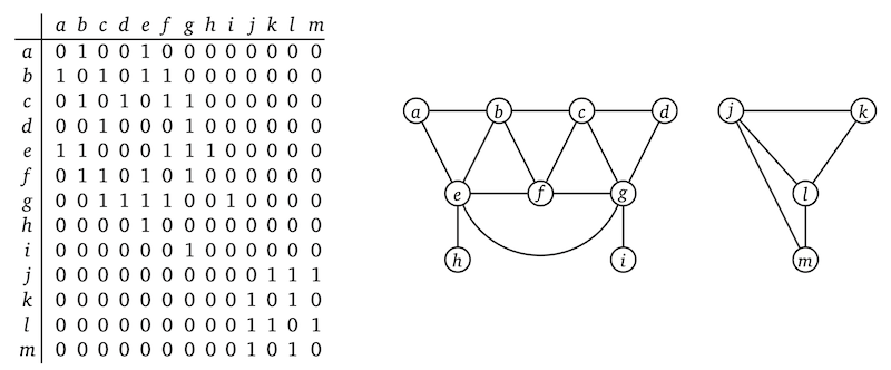Checking if uv \in E takes O(1) time. However, finding all neighbors of u takes O(|V|) time, because we have to scan u’s whole row. Also, we’re using O(|V|^2) space, even there aren’t any edges.

The default data structure we’ll actually work with is the adjacency list. You have a 1D array indexed by the vertices. The entry for each vertex u is a linked list of vertices v for which there is an edge u \to v or uv. 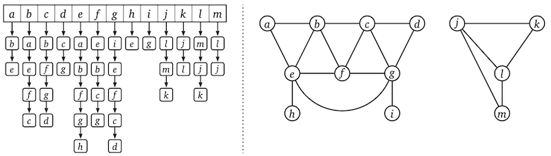Now, checking if u \to v \in E takes O(\mathit{deg}(u)) time, because we have to traverse u’s list. If G is undirected, we can check if uv \in E in O(\min (\mathit{deg}(u), \mathit{deg}(v))) time, by checking both lists in parallel and stopping when we read the end of the shorter one. However, we can iterate over the neighbors of u in constant time per edge. Also, this data structure it uses an optimal O(|V| + |E|) space, because we only see each edge represented at most twice.

Again, we’ll be using adjacency lists by default, and you should assume any abstract graph proposed in lecture or homework is stored using one unless we say otherwise. But that’s fine, because adjacency lists are typically how graphs you find in practice are implicitly represented. For dependency, configuration, and state-transition graphs, going through the ways to leave a subproblem, configuration, or state is the same as walking down one of the linked lists for a vertex.

It’s less common, but adjacency lists implicitly come up as well. For an intersection graph, you’ll typically check whether two objects intersect one at a time like checking entries in the matrix.

Whatever-first search

Alright, it’s time to discuss our first, and arguably most important, non-trivial graph algorithm. This algorithm is used to determine reachability: given a graph G = (V, E) and a vertex s \in V, which vertices v can be reached from s, i.e., for which vertices v is there a path from s to v? In an undirected graph, these are precisely the vertices in s’s (connected) component.

You’ve probably seen a couple of different algorithms that successfully solve this problem. But while these algorithms tend to be presented as their own things, they’re really all variants of the same algorithm. The main idea is that every time we “discover” a new vertex u is reachable from s, we should remember to follow its outgoing edges to find more vertices that can be reached from u. To that end, we put u into an arbitrary data structure (which I’ll call a bag) that supports insertion of a given element and pulling of an arbitrary element previously inserted. There’s a risk that we keep inserting the same vertex u over and over again, so after the first time we remove it, we’ll “mark” it to say there’s no need to ever put it back.

Depending on what data structure we choose for the bag, we’ll end up discovering and marking reachable vertices in different orders. You’ll end up with different [priority] first searches. Since the order doesn’t matter at this point, I’ll call the general strategy a whatever first search.

Here’s what the code might look like for a directed graph. It assumes all the vertices including s start as unmarked.

I claim \text{WhateverFirstSearch}(s) marks every vertex reachable from s and nothing else. A full proof of this claim appears in the book, and I recommend you look it over carefully, because it shows off a style of inductive proof that’s very common with graph algorithms. In short:

• If a vertex v gets marked, it’s because we added it to the bag after marking a vertex u, and we may assume inductively that u is reachable from s. There is a path from s to u and then through u \to v to v.
• On the other hand, if v is reachable, then we may inductively assume a closer to s neighbor u of v gets marked. After which, we will explore edge u \to v and add v to the bag to later be marked if v hasn’t been already.

Now, the exact order in which we mark vertices is affected by the bag we choose, and so is the running time. Suppose it takes T time to insert a vertex into or take a vertex from the bag. Each vertex is marked at most once, so we run “mark u” at most |V| times. Also, we look at each edge u \to v at most once, during the for loop immediately after marking u. Therefore, including the first line of the algorithm, we do at most |E| + 1 insertions into the bag. Finally, to remove a vertex u from the bag, we must first put it into the bag. Therefore, we take a vertex from the bag at most |E| + 1 times. Adding everything up, the total running time is O(|V| + T|E|). If we use, say, a queue or a stack for the bag, then T = O(1) and the running time becomes O(|V| + |E|). If you want to make a call \text{WhateverFirstSearch}(s) as a subroutine in homeworks or exams (and you will), you may assume it 1) marks all vertices reachable from s and 2) runs in O(|V| + |E|) time.

It’s also important to note that WhateverFirstSearch can be modified to handle undirected graphs by only looping over the edges uv incident to any vertex u. The running time remains the same.

Reductions: Useless state elimination

We can already solve a lot of new problems by reducing to graph reachability and performing whatever-first search. Here is one example involving some material earlier in the semester.

Suppose you’re given a DFA M = (Q, \delta, s, A) with n = |Q| states over the binary alphabeta \Sigma = \{0, 1\}. We’ll call a state q \in Q useless if there does not exist an input string taking M to q, i.e. there does not exists some x \in \Sigma^* such that \delta^*(s, x) = q. Our goal is to find all the useless states so we can remove them from the DFA.

For example, earlier this semester, we showed that for every NFA, there is a DFA accepting the same language. When we applied the standard construction to the example NFA (top image below) accepting all strings containing 00 or 11, we got the following DFA (bottom image below).

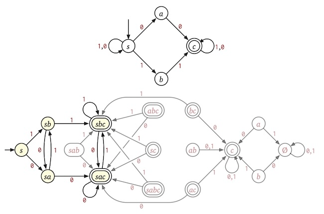
All of the grayed out states are useless, and we’d like to find them.

We can solve our problem by reducing useless state discovery to reachability. Let G = (V, E) be a directed graph over the states Q where there is an edge p \to q if and only if there is a symbol taking p to q. More concisely:

• V = Q and
• E = \{p \to q \mid \text{$\delta(p, 0) = q$ or $\delta(p, 1) = q$}\}.

Chasing definitions and a bit of straightforward induction (which I’m not going to do here, and I don’t expect you to do on homework solutions) implies there is a path from s to q in G if and only if q is not useless. Therefore, we should call \text{WhateverFirstSearch}(s) and report as useless every vertex q that is not marked.

That’s the algorithm, but how long does it take? We have |V| = n and |E| = 2n. Both building graph G and running \text{WhateverFirstSearch} (with a stack as the bag) take O(|V| + |E|) time. However, neither V nor E are given as part of the problem description. In terms of the original input, we should say the algorithm takes O(|V| + |E|) = O(n) time.

Notice how I did a few things here when I described this reduction that you’ll have to do as well.

1. I described exactly what graph to construct including specifying its vertices and edges.
2. I said what problem we need to solve in the graph including specifics about its input such as the starting vertex s.
3. I said what algorithm to run to solve the problem, again including it’s full input.
4. I analyzed the running time in terms of the input to our original problem and not just the number of vertices and edges in the graph we made up.

All of these steps are described in detail in the standard grading rubric on the course website and in less details at the beginning of tomorrow’s lab handout. Please look them over.

Graph layering: walks of length divisible by 3

We’ll finish by solving a problem on graphs that is best solved by doing a reduction to a different problem in a different graph.

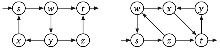
We’re given a directed graph G = (V, E) and two vertices s and t. We want to determine if there is a walk (possibly repeating vertices and/or edges) from s to t whose length is divisible by 3. For example, the graph on the left has such a walk s \to w \to y \to x \to s \to w \to t. The graph on the right has infinitely many walks from s to t, but none have length divisible by 3.

This feels like graph reachability, so many of you may be tempted to modify WhateverFirstSearch to, say, keep track of how many steps you’ve taken (mod 3) as you add a vertex to the bag. In principle, this strategy can work, but it’s really hard to get it right, especially in this case where we’ll want to walk through the same vertex up to 3 times. So instead, we’re going to do a reduction to plain WhateverFirstSearch in a directed graph. It just won’t be the same graph we were given.

Imagine you’re an ant wandering around the graph trying to find a walk from s to t of length 0 \mod 3. What information do we need to maintain? How about:

• The current vertex, so we know what edges are available and whether we’ve gotten to t.
• How many edges we’ve traversed (mod 3), so we know if we’ve succeeded when we reach t.

We’ll play a trick similar to the one we played when designing NFAs for language transformations: we’ll have the new graph track both a vertex of the input graph and a counter for how many edges we’ve walked mod 3. We construct a layered graph G' = (V', E') where

• V' = \left\{(v, i) \mid v \in V \text{ and } i \in \{0, 1, 2\}\right\}, and
• E' = \left\{(u, i) \to (v, i + 1 \mod 3) \mid u \to v \in E \right\}.

In other words, G' contains three copies of every vertex in G. Each choice of i \in \{0, 1, 2\} defines a “layer” of vertices (v, i), and for every edge u \to v \in E, there are edges going from u in each layer to v in the “next” layer (mod 3).

Some straightforward definition chasing (and, again, induction) suggest that for each i \in \{0, 1, 2\}, there is a bijection between walks from u to v of length \ell \mod 3 in G and walks from any (u, i) to (v, i + \ell \mod 3) in G'. In particular, G' contains a walk from s to t of length divisible by 3 if and only if G' contains a walk from (s, 0) to (t, 0).

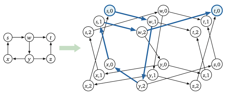
For example, the input graph on the left transforms as follows. The thick blue vertices and edges show a path from (s, 0) to (t, 0) in the new layered graph.

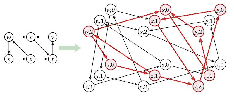
And here’s the input graph on the right being transformed. There is no walk from (s, 0) to (t, 0) to show off. Instead, the thick red vertices and edges show all the vertices in the layered graph reachable from (s, 0).

Now that we’ve built our layered graph G', all that remains is to run \text{WhateverFirstSearch}((s, 0)) in G' and return True if and only if (t, 0) gets marked.

Graph G' has exactly 3|V| vertices and 3|E| edges, so we may construct it in O(V + E) time. Combined with the time to run WhateverFirstSearch, the whole thing takes O(3V + 3E) = O(V + E) time.