Divide-and-Conquer

Quickersort

Last time, we saw quicksort, a recursive sorting algorithm that included a call to a procedure called \text{Partition}.

\text{Partition}(A[1~..~n], p) would take the element at position/index p and rearrange the members of A so everything less than p went to its left and all other elements went to its right. It then returns the new index r of the element, its rank.

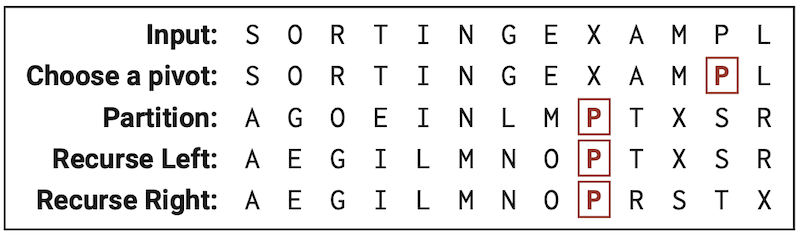
Despite its name, though, quicksort holds a dark secret; its worst case running time is based on the recurrence T(n) = \Theta(n) + \max_{1 \leq r \leq n} \left(T(r - 1) + T(n - r)\right), and by setting r to be 1 or n, we see T(n) \geq \Omega(n) + T(n - 1), implying T(n) = \Omega(n^2).¹ Why would we even call this thing quicksort?

I believe most people tend to imagine the following scenario. Suppose r = n / 2. Then, T(n) = O(n) + T(n/2) + T(n/2) = O(n \log n).² This scenario is unrealistically optimistic, even “in practice”. However, you will (probably, if you trust the users of your algorithm) get a pivot that lies near the middle of the array. Suppose n/3 \leq r \leq 2n/3. In this scenario, T(n) = O(n) + \max_{n/3 \leq r \leq 2n/3} (T(r - 1) + T(n - r)). To keep things clean, I’m going to make the (correct) claim that this recurrence is maximized when r = n/3 or r = 2n/3, leading to a recurrence of T(n) = O(n) + T(n/3) + T(2n/3). Now we get the following recursion tree:

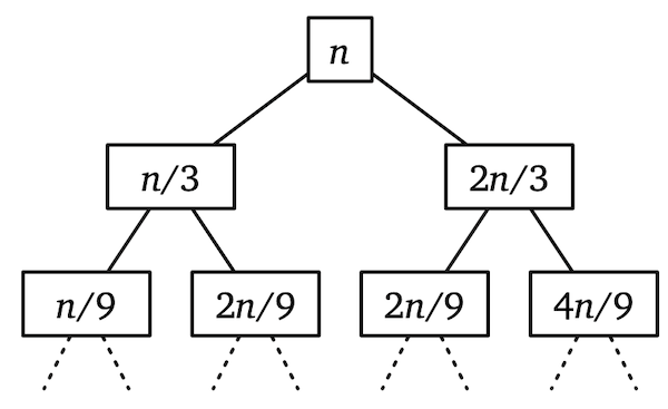
Each level still sums to at most n. However, even following the chain of larger subproblems, we see the depth of the tree is at most \log_{3/2} n. The running time is O(n \log n) like in the ideal case!³ If only there was a way to select such a good pivot…

Selection

Well, maybe we can find an algorithm for that problem. Specifically, let’s see if we can find the median of the array A[1~..~n], which for this class is defined as the element of rank \lceil n/ 2 \rceil. We’re in a recursion mood, so what might be useful is to first identify some smaller subset of elements that must contain the median, or equivalently, find a subset that cannot contain the median. And we already have a procedure for subsets of elements based on rank: \text{Partition}.

So let’s pick a pivot A[p], call \text{Partition}(A[1~..~n], p), and then recursively search something based on the resulting array. \text{Partition} returns the rank r of the pivot. If r = \lceil n / 2 \rceil, we’re done. If it’s too large, we need to search in the left subarray, and if it’s too small, we need to search in the right subarray.

But how do we search the smaller subarray? Using recursion of course. And that means calling an instance of the same… problem. Oh no. The median of A[1~..~n] isn’t the median of either subarray. It may have a different rank relative to the subarray.

Fortunately, we can compute the rank of the input array’s median within the smaller subarray. So maybe that’s the problem we should be solving recursively? Given A[1~..~n] and an integer k such that 1 \leq k \leq n, we want to find the element of rank k. We call this new problem selection.

The following algorithm for selection was also found by Tony Hoare and it appears on literally the same page of paper as quicksort.

Observe how when doing the recursive call on the latter subarrary A[r + 1~..~n], we have to reduce the rank of the element we’re looking for. After all, there are r elements from A of lessor rank that aren’t part of that recursive call.

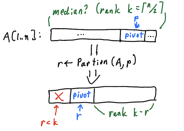
So what’s the running time? Well, it again depends upon r but also which recursive call we make, so T(n) \leq O(n) + \max_{1 \leq r \leq n} \left(\max\{T(r - 1), T(n - r)\}\right). And, uh, assuming T is increasing, T(n) \leq O(n) + T(n - 1) = O(n^2). Oh. We’d be better off running Mergesort and then returning the kth element.

But what happens in our moderately optimistic scenario n/3 \leq 2n/3? Now the subproblems have size at most 2n / 3, so T(n) \leq O(n) + T(2n / 3). A quick look at the recursion tree path, shows the solution is O(n). We can’t do better than that (assuming the array isn’t presorted or something).

It seems our attempt to find the median element quickly has been reduced to finding something near the median. And yes, that sounds like a job for recursion, but its unclear what kind of subproblem we can work with.

Blum, Floyd, Pratt, Rivest, and Tarjan figured out the solution the early 1970s. The idea is to find a representative sample of the elements in A and take their median, with the hope that it’s rank in A is somewhere near n/2. The sample they chose to work with to find something near the median is… a bunch of other medians.

We divide the input array into \lceil n / 5 \rceil blocks, each with exactly 5 elements (and we can throw in a few \inftys to pad the last one if necessary). Then we compute the medians of the blocks in constant time each using brute force, and we put those medians into a new array M\left[1~..~\lceil n/5 \rceil\right]. And to compute the medians of those medians, we use recursion!

And now we’ve made a huge mess by doing two recursive calls on to likely overlapping subsets, one of which has who knows what size. And here’s how to become one who knows.

For simplicity, I’ll assume no two elements are equal. So first, imagine that we (for the sake of proof—not in the algorithm) rearrange A’s elements into a 5 \times \lceil n/5 \rceil grid where each column is one of our blocks of five. Now sort each individual column so its elements go in increasing order from top down. The mediums of each block appear in the middle row. And now, sort the columns from left to right according to their middle/median element. The median of medians appears in column \left\lceil \lceil n/5 \rceil / 2 \right \rceil \geq n/10.

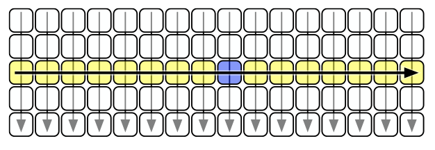
If we look in any one column at or to the left of the median column, each of its first three elements is at most its own median and therefore at most the median of medians. Therefore, that are at least 3 \cdot (n/10) = 3n/10 elements smaller than the median of medians, and therefore, there are at most n - (3n/10) = 7n / 10 elements greater than the median of medians. If we have to recurse on the greater element subproblem, it has size at most 7n / 10.

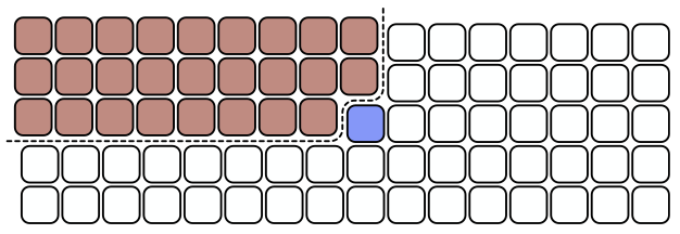
A symmetric argument suggests the smaller element subproblem also has at most 7n / 10 elements. So either way, our second recursive call is on an input of size at most 7n / 10, and our first recursive call is on \lceil n/5 \rceil elements by design. The recurrence for the run time is T(n) = T(n/5) + T(7n/10) + O(n). We have another unbalanced recursion tree.

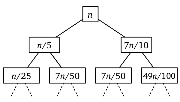
Each level i sums up to at most (9/10)^i n. The sum of level sums is a decreasing geometric series asymptotically equal to its largest term. T(n) = O(n).

Karatsuba multiplication

I have a kid who (at the time I’m writing this note) is in elementary school. And, I’m afraid to say, he hates doing arithmetic in his homework, especially tedious stuff like “long” multiplication.

And that’s fair! It’s a long boring grind as demonstrated by this example from Wikipedia:

      23958233
×         5830
———————————————
      00000000 ( =  23,958,233 ×     0)
     71874699  ( =  23,958,233 ×    30)
   191665864   ( =  23,958,233 ×   800)
+ 119791165    ( =  23,958,233 × 5,000)
———————————————
  139676498390 ( = 139,676,498,390)

You have to take each digit from the number on the bottom and multiply it by the entire number on the top, shifting the result of each one digit by x digit multiplication one additional unit to the left. Then, you add up all the numbers you just made.

Fortunately, my son’s problems tend to have only three or four digits, but if there were, say, n digits in both numbers, it would take him O(n) time per digit in the bottom number and O(n^2) time overall.⁴

There’s got to be a better way! And of course the answer has to involve recursion somehow if I’m bringing it up today.

Let’s try a divide-and-conquer approach. Say we have two numbers x and y, each of n digits. We can split each of their digits up into two nearly equal halves. Let m = \lceil n / 2 \rceil. Let a be the more significant n - m digits of x, let b be the less significant m digits of x, let c be the more significant n - m digits of y, and let d be the less significant m digits of y.

To summarize, we have: \begin{align*} m &= \lceil n / 2 \rceil \\ x &= a \cdot 10^m + b \\ y &= c \cdot 10^m + d \end{align*}

A bit of algebra shows us xy = (a \cdot 10^m + b)(c \cdot 10^m + d) = ac \cdot 10^{2m} + ad \cdot 10^m + bc \cdot 10^m + bd.

Hey, those are products of smaller numbers, so we can find them using recursion.

The \text{SplitMultiply} procedure below takes two integers x and y, each with at most n digits, and returns x \cdot y.

We can do addition of two n-digit numbers in O(n) time, and multiplying a number by 10^k for some integer k < n also takes O(n) time (just add k 0s), so the non-recursive work takes O(n) time total. The total time to do the multiplication can be expressed by the recurrence T(n) = 4T(n / 2) + O(n).

Here’s the recursion tree for the recurrence:

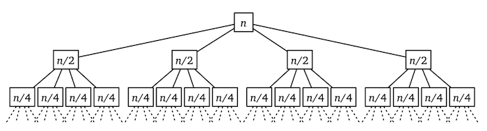
The level sums seem to be increasing. In particular, the node values at level i sum to 4^i \cdot (n / 2^i) = 2^i n. That’s an increasing geometric series, proportional to its largest term and it’s largest term depends upon the depth, \log_2 n.

There are two ways we can compute the largest term. The first is to plug the depth into the expression we just gave for the ith level sum. \begin{align*} 2^{\log_2 n} \cdot n \\ &= n \cdot n \\ &= n^2 \end{align*}

The other method (and the one I find a bit easier algebraically) is to recognize that every leaf in the tree has value (some constant times) 1. There are 4^{\log_2 n} = n^{\log_2 4} = n^2 leaves where the first equality comes from the fact that a^{\log_b c} = c^{\log_b a} for any a, c > 0 and b > 1.

Either way, T(n) = O\left(2^{\log_2 n} \cdot n\right) = O(n^2).

Oh. That didn’t help after all. And until the 1960, most people thought O(n^2) was the best you could do. Karatsuba had a great observation, though. We need to compute ad + bc and multiply this sum by 10^m (given as g and h in the pseudocode above). However,⁵ \begin{align*} ad + bc &= (ac + bd) + (-ac - bd + ad + bc) \\ &= ac + bd - (ac + bd - ad - bc) \\ &= ac + bd - (a - b)(c - d) \end{align*} Oh! We were already computing those first two terms, and the third term is a single product of two numbers with at most m digits each. We can compute x \cdot y using only three recursive calls.

Now, T(n) = 3T(n / 2) + O(n), and we get a different recursion tree:

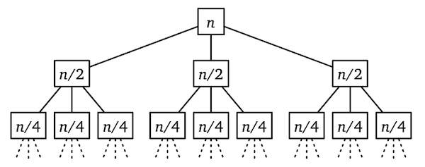
The node values at each level i now sum to (3/2)^i n, and there are still \log_2 n levels in the tree. We need to know the sum at the lowest level which we can compute using the formula: \begin{align*} \left( \frac{3}{2} \right)^{\log_2 n} \cdot n &= n^{\log_2 \frac{3}{2}} \cdot n \\ &= n^{(\log_2 3) - 1} \cdot n \\ &= n^{\log_2 3} \end{align*}

Or we can more directly observe that the number of leaves is 3^{\log_2 n} = n^{\log_2 3}.

Either way,⁶ T(n) = O\left(n^{\log_2 3}\right) = O(n^{1.59}) = o(n^2).

That’s much better for large values of n.

There was a long sequence of improvements after this particular result based on splitting the numbers into more and smaller parts while also doing more and more multiplications (see Erickson’s Algorithms Exercise 1.22 for how to specifically apply this idea to squaring a number). A 1971 method based on the fast Fourier transform leads to an O(n \log n \log \log n) time algorithm. You can learn more about Fast Fourier transforms in CS 473 (and probably some ECE and CS classes involving networking or signal processing).

After a long period of time and a few technical improvements that all came very recently, we finally got an O(n \log n) time algorithm in 2019. It is absolutely not worth running in place of the 1971 algorithm, because you’d need more digits than there are particles in the universe to actually see the time improvement. But why should that stop us from doing cool math?