Depth-first Search

WhateverFirstSearch variants and spanning trees

We’ve now seen an example of how reducing to reachability is already enough to do something practically useful and an example of a more complicated reachability-like problem that can be solved by reducing to standard reachability. However, the basic reachability problem only asks if a vertex s can reach a vertex v. There no concern about how we find that vertex or what path leads to it.

Often, though, you actually do care about how you found a vertex. For the first consideration, it’s helpful to consider this slight variant of the WhateverFirstSearch procedure which puts whole edges into the bag. Let G = (V, E) be a (directed) graph and s \in V be a vertex.

Now when we remove something u \to v from the bag, we get the entire edge used to discover v (the very first time we pull, we get \bot \to s, representing us not having to use an edge to reach s).

With this variant of the algorithm, we still mark exactly those vertices v that are reachable from s. However, we also record which edge p \to u led to u’s discovery (unless u = s, in which case we record that no edge was needed). For each marked vertex except for s, there is exactly one edge v.\mathit{parent} \to v. These edges form a rooted tree with s as its root. If G is undirected, this the tree is a spanning tree of s’s component.

We saw last time that the choice of bag affects the running time of the algorithm. Specifically, a bag with T time insertion and removal leads to an O(|V| + |E|T) WhateverFirstSearch. The choice of bag also affects the kind of rooted tree you might get, and these differences are important enough that we typically give the resulting algorithm a different name for each fixed choice of bag. We’ll survey a couple of “natural” choices for the bag.

Queue: breadth-first search

Suppose we want to explore from vertices in the order we first discover them. We can do so with a queue, resulting in a breadth-first search (BFS). The parent edges form a breadth-first search tree containing the shortest unweighted paths from s to every reachable vertex. Queues have O(1) time insertion (enqueue) and removal (dequeue), so BFS takes O(|V| + |E|) time.

Priority queue: best-first search

Alright, but what if we want to prioritize what we search for in another way. In this case, we might use a priority queue. We call the resulting family of algorithms best-first search, because we keep taking the best choice but what “best” means is still dependent on how we set the priorities. The time needed is going to be the same in each case, however. The bag always contains at most |E| edges which is O(|V|^2) assuming G is simple. Using a standard binary heap (which is a particular implementation of priority queue), each bag operation takes O(\log |E|) = O(\log |V|) time, and the whole algorithm takes O(|V| + |E| \log |V|) time. Let’s consider two best-first searches. For both, we’ll assume each edge u \to v or uv has a non-negative weight w(u \to v) or w(uv). We’ll consider what priority to assign when adding (u, v) to the priority queue.

Going along with the BFS example, suppose we set the priority of (u, v) to the length of the tree path from s to u plus w(u \to v). In this case, we compute a shortest paths tree containing shortest paths from s via what is essentially Dijkstra’s algorithm.

Another option is only really useful if G is undirected. In that case, if we use the weight of the edge w(uv) as the priority of (u, v), then we end up computing a minimum spanning tree via what is essentially Prim’s algorithm.

Stack: depth-first search

The final variant we’ll consider is using a stack for the bag. Doing so results in a depth-first search (DFS) creating a breadth-first search tree. Stacks have O(1) time insertion (push) and removal (pop), so DFS takes O(|V| + |E|) time. But why would you want such a thing? That requires more explanation…

DFS in detail

Unlike the rest of the algorithms “unit” where I state a problem and then work toward an algorithm to solve it, we’re going to study the specific algorithm DFS in more detail and see what problems can be solved using it. It turns out that a lot of problems benefit from using a DFS, but we only have so much time, so I’ll focus on just a few and the subset of facts about DFS we need to solve them.

While DFS is really another variant of WhateverFirstSearch (WFS), it will help to look at it written in a different way. First, observe that when WFS is looping over edges leaving some vertex u, then last edge u \to v seen is the first one popped from the stack. We’re going to immediately start working with v, so why not make that more explicit by beginning the search from v recursively. Second, we’ll check if a vertex v is unmarked before we do its recursive call, because the call would have returned immediately otherwise.

As with any WFS, the top-level call \text{DFS}(s) will end up marking all vertices reachable from s. However, different choices of s will result in marking different vertices. This phenomenon happens even if the graph is merely a path; the first vertex can reach every other vertex, but the last vertex can only reach itself. Most applications of DFS aren’t just about what a single vertex s can reach, though; they’re more about how to reach different vertices and in what order, and in most of these applications, we’d like to learn about every vertex in the graph.

To that end, we’re going to introduce another procedure called DFSAll that iterates over every vertex v in the graph, calling \text{DFS}(v) whenever it encounters a vertex that has yet to be marked. When the procedure ends, every vertex will be marked, meaning we called \text{DFS}(v) on every vertex at some point. ¹

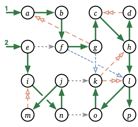
Below is an example of what running DFSAll might look like assuming all the for loops go over vertices in alphabetical order. The dark green edges are those in the rooted trees found by DFS. In this example, DFSAll successfully makes exactly two direct calls to DFS, indicated with the numbered edges with no tail/predecessor vertex. You can safely ignore the various colors and designs on the other edges in the graph.

All the direct applications of DFS we’ll see today use variants of DFS and DFSAll as given above, and everything continues to run in O(|V| + |E|) time. We can make a few observations right away that will help us in these applications.

1. Every vertex of G is eventually marked. This fact is guaranteed by the second for loop in DFSAll.
2. Suppose a run of \text{DFSAll}(G) (indirectly) calls \text{DFS}(v). For each vertex w reachable from v without going through a marked vertex, an instance of \text{DFS}(w) will run before \text{DFS}(v) finishes.
3. In particular, if a call \text{DFS}(v) (indirectly) calls \text{DFS}(w), then there is a path from v to w in G.

Preorder and postorder

The next change I’m going to show if purely to help us understand the behavior of these algorithms.

The big idea here is that the applications we’re interested in are largely based on the relative order in which start and finish the recursive calls on the various vertices, and we need some way to track that order. To that end, I’m going to introduce an integer variable \mathit{clock} that starts at 0 and change the interface of \text{DFS} to take as parameters both a vertex v and the current value of the clock. As DFS runs, it will increment the clock a few times and then return its new value. We’re going to use the clock to track the start time of each vertex v, defined as its clock value when \text{DFS}(v) has just begun, and its finish time, define as the clock value when \text{DFS}(v) is about to end. These will be stored in v.\mathit{pre} and v.\mathit{post}, respectively.

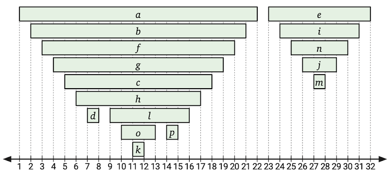
For a given run of DFAAll, we’ll say the active interval for a vertex v is [v.\mathit{pre}, v.\mathit{post}]. If \text{DFS}(u) calls \text{DFS}(v) (either directly or indirectly), then the call to \text{DFS}(v) has to end before the call to \text{DFS}(u) can end. Therefore, pairs of active intervals are either disjoint or nesting. The figure below shows the active intervals for the DFSAll call shown above.

If we order the vertices by their start times (v.\mathit{pre}), we get a preordering of the vertices. These actually aren’t all that useful! However, if we order the vertices by their finish times (v.\mathit{post}) we get a much more useful postordering of the vertices.

Note: There may be several preorders and postorders of a single graph. It all comes down to the arbitrary order in which DFSAll and DFS calls iterate over their vertices and edges.

Dependency graphs and dags

We’re going to motivate the rest of the discussion and the applications of DFS by focusing on a specific use of graphs. Recall, every instantiation of a recursive algorithm leads to a directed dependency graph where vertices are subproblems that must be solved while running the algorithm and there is an edge u \to v whenever subproblem u does a recursive call to subproblem v. For example, here is the dependency graph for computing the nth Fibonacci number recursively.

For the algorithm to terminate, the dependency graph cannot contain directed cycles; if there is a cycle containing a vertex u, then completing the subproblem for u would require first completing the subproblem for u! So that motivates our first application.

Detecting cycles

Given a directed graph G = (V, E), we’d like to know if it contains any cycles. A directed graph with no directed cycles is called a directed acyclic graph or dag. Because they tend to be important, we call a dag vertex with no incoming edges a source and one with no outgoing edges a sink.

Imagine running DFAAll. You’re several recursive calls deep into a running \text{DFS}(v) and during a subcall to \text{DFS}(u), you discover edge u \to v. We call such an edge u \to v a back edge. There’s a path from v to u (Observation 3. above). Combined with edge u \to v, we have a directed cycle! Lemma: If \text{DFSAll}(G) encounters a back edge, then G has a directed cycle.

It’s intuitively feasible, though, that a cycle could exist but we don’t find a back edge. Perhaps we call DFS on one of the cycle’s vertices, but others are already marked so we never manage to explore all the way around. That concern doesn’t actually come up, though!

Lemma: If G has a directed cycle, then \text{DFSAll}(G) encounters a back edge.

So that’s one method of determining if a graph has no cycles; check if there’s a back edge. There’s pseudocode based on that idea in the book, but there’s an even easier approach that doesn’t require opening the DFS black box. If u \to v is a back edge, then \text{DFS}(v)’s active interval encloses that of \text{DFS}(u), implying v.\textit{pre} < u.\textit{pre} < u.\textit{post} < v.\textit{post}. Active intervals don’t properly intersect, and \text{DFS}(u) will try to directly call \text{DFS}(v) if v is not already marked, so u \to v being a back edge is the only way for there to be an edge u \to v while u.\mathit{post} < v.\mathit{post}. Putting everything together: Lemma G has a cycle if and only for some edge u \to v, we have u.\textit{post} < v.\textit{post}.

We can detect if there’s a cycle (and we don’t have a dag) in O(|V| + |E|) time by running DFSAll and seeing if u.\textit{post} < v.\textit{post} for any edge u \to v.

Memoization and topological sort

Going back to our motivation of studying dependency graphs. Suppose we know (or verify using the previous algorithm) that a dependency graph G is a dag. That highly suggests its algorithm will terminate, but it may not be fast. To guarantee it runs quickly, we’d like to memoize the solutions to the subproblems for dynamic programming. But what order do we solve the subproblems in?

What we want is a topological ordering of the reversal of the dependency graph. A topological ordering of a directed graph G is a total order on the vertices where u comes before v if there’s an edge u \to v. In other words, we can place all the vertices on a horizontal line so that every edge is directed left-to-right. As argued earlier, a topological order can only exist if G is a dag.

But what if there are no cycles? Then in a run of DFSAll, there are no back edges. Meaning u.\mathit{post} > v.\mathit{post} for every edge u \to v. The reversal of a postorder is a topological ordering! So if we want to compute one, we can do so in O(|V| + |E|) time by using DFSAll to compute a postorder and reversing the postorder.

As for dependency graphs, we’d like to memoization in topological order of the reverse graph, and through essentially the same argument, that means we should solve the subproblems in postorder. We’ll return to that idea next week.