Backtracking

n queens

For the next two weeks, we’ll be going what is arguably the most powerful method we have for designing correct and efficient algorithms. However, it’s incredibly easy to write incorrect algorithms while claiming to use this method, so we’re going to take things in stages.

First, we’ll make it work, and then we’ll make it fast.

The key to making it work is a recursive algorithm strategy called backtracking. In this strategy, you model solving your problem as making a sequence of decisions. For each option for the current decision (and only that one decision), you do a recursive call based on the consequences of that one decision (and, in accordance with the recursive problem definition, any relevant previous decisions).

To demonstrate this strategy, we’re going to consider the following problem: We’re given an n \times n chess board upon which we’re going to place queens. We say two queens attack one-another if they lie in the same row, column, or diagonal of the board. Our goal is to determine every way of placing exactly n queens so that no pair of them attack one-another. Here is one solution to the standard 8 \times 8 version:

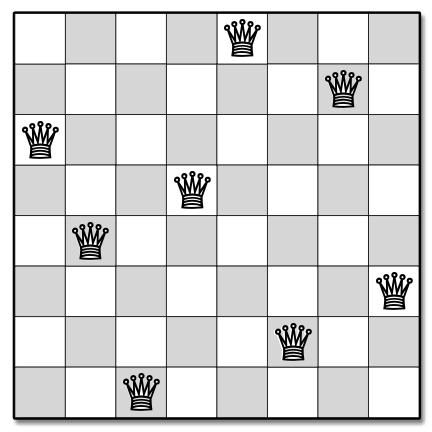
To represent our solutions, we’ll have our algorithm “print” several arrays Q[1~..~n], one per solution, that tell us to place the queen for row r in column Q[r]. Rows are numbered from 1 to n from top down, and columns are numbered from 1 to n going left to right.

So how do we handle this problem? Let’s think of it as a sequence of decisions. In particular, each row receives exactly one queen in a valid solution, so let’s guess where the queen for each row r goes row by row from top down.

Suppose we’re trying to decide where to place a queen in row r with 1 \leq r \leq n. We’ll look at every square j in that row and decide if we can place a queen there. If the square is already being attacked by a queen in higher row r' < r, we cannot use it, and so we don’t. However, if row r square j is not being attacked, we can maybe place the queen in a valid solution. We don’t know yet if we should, though, or how many solutions exist that use that particular spot for the queen. Regardless, we try the placement and then ask the Recursion Fairy to print solutions that are based on where we put queens in rows 1 through r (which includes the new queen we’re tentatively trying out). Again, we do this recursive call (if it makes sense to do so) for every column j.

Below is pseudocode based on the idea. The procedure \text{PlaceQueens}(Q[1~..~n], r) prints all arrays of valid placements as described above assuming positions Q[1~..~r-1] are already decided upon and no queens within those row attack one-another. In the base case of r = n + 1, it’s given all the placements and can immediately print. Otherwise, it applied the above strategy. To solve the problem from scratch, we call the procedure with r = 0.

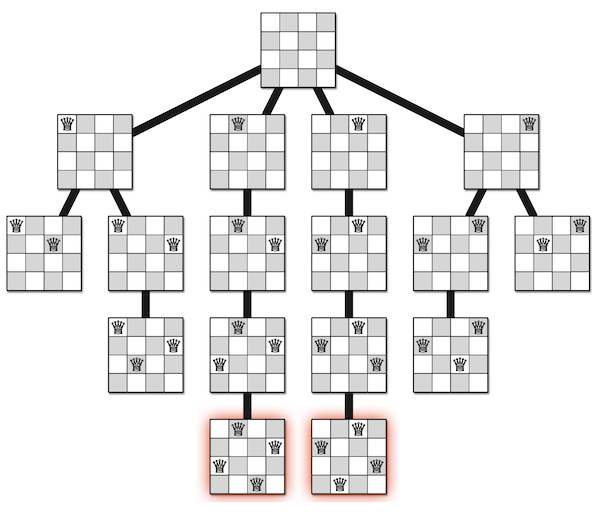
It might help you see what is going on to look at the recursion tree for an instance of this algorithm. Unlike when we were analyzing divide-and-conquer algorithms, we’re not writing running times into our recursion tree nodes. Instead, each node is going to display the current state of the board during its call. Any node at depth n is a leaf whose board gets printed. Any leaf node at a depth r - 1 < n represents board with guessed queens in the first r - 1 rows that attack every square in row r. As shown in the figure below, the n = 4 queens problem has only two solutions.

Text segmentation

Suppose we’re given a string of letters representing text but without and spaces or punctuation.

We’d like to break this string into its individual component words or (for the purposes of easy class example) simply determine if it is possible to do so. To get around minor issues like “what is a word?” we’ll assume we have access to a subroutine \text{IsWord}(w) that takes a string w as input and returns \text{True} if w is a “word” (according to whatever language or other restrictions we have) or \text{False} otherwise.

We’ll try a backtracking approach. Which means we should thinking about solving this problem as a sequence of decisions.

A string is itself a sequence, so one strategy we might consider is to decide what to do with each individual character one by one. In principle, we could make a backtracking algorithm based on this idea, but it might get a little messy considering \text{IsWord} wants to take in entire words worth of characters as a time.

So instead, we’re going to make a sequence of decisions based on the sequence of words that make up some segmentation of the input string. We’re repeatedly ask, “What is the next word in the segmentation?” based on the words we previously decided might belong to a good segmentation. Each subsequent decision is based on the words chosen before it.

For example, suppose our input string is the following:

BLUESTEMUNITROBOTHEARTHANDSATURNSPIN

Partway through the algorithm, we may have decided we’re going to use the prefix of words “BLUE STEM UNIT ROBOT”.

BLUE STEM UNIT ROBOT HEARTHANDSATURNSPIN

Now we need to decide what the next word should be. And so we try every possible word beginning with that H right after ROBOT for our next decision. Assuming we’re working with English words in this example, we could take any one of HE, HEAR, HEART, or HEARTH.

How do we know which one to take? We try them all! For each of the possible words, we tentatively decide it should be the next one and let the Recursion Fairy tell us if there’s a segmentation based on what we’ve done already. If we take HE, then we recursely continue segmenting from

BLUE STEM UNIT ROBOT HE ARTHANDSATURNSPIN.

If we take HEAR, then we recursely continue segmenting from

BLUE STEM UNIT ROBOT HEAR THANDSATURNSPIN.

If we take HEART, then we recursely continue segmenting from

BLUE STEM UNIT ROBOT HEART HANDSATURNSPIN.

If we take HEARTH, then we recursely continue segmenting from

BLUE STEM UNIT ROBOT HEARTH ANDSATURNSPIN.

No, we don’t try to be clever with which one or more choices to try. To be clever would require us to know and explain how we know some words are better than others. Yuck. That’s too much thinking. Instead, we try them all!

If the Recursion Fairy says that even a single one of our tentative choices works, then we say Yes, we can segment the string.

Now that we have a strategy in mind, we need to specify exactly what problem we’re asking the Recursion Fairy to solve. For n queens, we needed to provide a row number and a list of all queen placements for the higher rows. For text segmentation, however, our previous choices of words have relatively little effect on future decisions beyond reducing the number of characters left to segment. All the Recursion Fairy needs to know is the suffix of the input string that still needs to be segmented.

Finding the correct recursive subproblem is usually the most difficult and most important part of designing a correct backtracking algorithm.

Now that we know what shape our recursive subproblem has, and only now that we know the right shape, we should handle base cases. The only time our strategy of guessing a next word doesn’t make sense is when dealing with the empty suffix, and that case is trivial: the empty string can be segmented into a sequence of zero words!

We’re finally ready to describe our recursive algorithm for (deciding if we can do) text segmentation. The following procedure takes in an array A[1~..~n] of characters and returns whether or not they can be segmented into words accepted by the \text{IsWord} function.

Preparing to make it fast

We’ve now seen a couple of examples of backtracking algorithms, but we haven’t even bothered to discuss running time. That’s intentional. We need to understand how to make correct algorithms before we can make fast ones. We won’t see the full strategy for speeding them up in this lecture, but I will describe something that will help make the basic backtracking text segmentation algorithm faster in practice while also setting things up to be easier on Thursday.

First, we don’t want to literally pass the input array around as an input parameter. In fact, for the purpose of describing an algorithm it’s actually helpful to treat it like a global variable.¹ But we do need something to pass around so we know what subproblem we’re working with. Fortunately, we’re not dealing with arbitrary subsequences of the input. Instead, they’re always suffixes and those can be described using a single index telling you where the suffix begins. In other words, the recursive subproblems we’re really trying to solve are:

Given the index i, is suffix A[i~..~n] the concatenation of words?

A direct pseudocode translation of our original algorithm based on passing only i around looks like the following. This procedure returns True if and only if A[i~..~n] is splittable.

There’s an even more concise way to describe this procedure that will serve us well in the next lecture. Because the input to the procedure \text{Splittable} is based on a single index i, we can treat it like a mathematical function and write what it does using mathematical notation. To that end, we might recognize that the inputs to \text{IsWord} are also based on indices relative to the input A. However, you need two indices to say where the potential word begins and ends.

In summary:

• Let \mathit{IsWord}(i, j) = \text{True} if and only if A[i~..~j] is a word and \text{False} otherwise.
• Let \mathit{Splittable}(i) = \text{True} if and only if the suffix A[i~..~n] can be split into words.

And now, based on the above recursive strategy, we can state that \mathit{Splittable} follows this recurrence:

\mathit{Splittable}(i) = \begin{cases} \text{True} & \text{if $i > n$} \\ \bigvee_{j = i}^n \left(\mathit{IsWord}(i, j) \wedge \mathit{Splittable}(j + 1)\right) & \text{otherwise} \end{cases}

(Here, \bigvee_{j = i}^n means doing a logical or over all choices of j, and \wedge means and.)

In particular, our original input array A[1~..~n] is splittable if and only if \mathit{Splittable}(1).

That recurrence expresses the exact same algorithm as the pseudocode given above. And while it just look like a notation hack, using this index notation instead of array notation can help us speed up backtracking algorithms (by removing the temptation to pass whole arrays around). It’s also going to help in deploying our main method of speeding up backtracking: dynamic programming.

Subset sum

For the last example in this lecture, we consider the SubsetSum problem: We’re given a set X of positive integers and a non-negative integer T. The goal is to decide if there exists a subset of X' \subseteq X such that \sum_{x \in X'} x = T.

For example, if X = \{2, 5, 8\} and T = 10, then we should report True, because 2 + 8 = 10. If X = \{2, 5, 8\} and T = 6, we should report False, because there is no way to take at most one of each of those integers so the sum is 6.

We need to think of this problem as making a sequence of decisions, and the most natural one I can imagine is to consider each element x of X one by one and decide whether or not x belongs to the subset we’re building.

Specifically, suppose we’ve built up a tentative subset Y \subseteq X based on our decisions so far, and we have Z \subseteq X elements left to make a decision on. Let z \in Z be any element we yet to make a decision on. If T - \sum_{y \in Y} y < z, then we have no choice to make. We cannot add z to Y and expect our sum to reach T (again, members of X are positive). Otherwise, we might take z or we might not, and the Recursion Fairy should handle both cases.

Now we need to figure out exactly what our recursive subproblems look like. The specific elements we’ve chosen to include already (given as Y above) don’t matter beyond limiting how much more we can add to the subset, and that “how much more” is easiest to represent as T - \sum_{y \in Y} y. We also need to know the full set of elements we have yet to consider (given as Z above). The previous observations suggest our recursive subproblems should be based on

• a (possibly new) target T, and
• a (possibly smaller) set of elements X.

All that’s left for finding a correct recursive backtracking algorithm is to handle base cases. The above strategy only fails to apply if there are no elements left to consider, i.e., X = \varnothing. In this case, there is a subset summing to T if and only if T = 0. Here’s the pseudocode for the above algorithm.

This algorithm is slow, because it may end up doing several recursive calls per each of the 2^{|X|} subsets of X. We can’t fully fix that problem in this lecture, but we can at least substantialy reduce the number of subsets while also using index notation to prepare us for the next lecture.

The trick is to recognize that we don’t need to consider every subset of X. In particular, we can decide on an ordering of the elements of X ahead of time, and go through this ordering from beginning to end as we make decisions on which elements to include in the subset.

Let’s assume our set of elements is given as an array X[1~..~n]. We’ll be going through the elements one by one, making recursive decisions based on what is left, so recursive subproblems will consist only of suffixes of X along with the target value that the suffix needs to sum to. We can use a single index i to denote which suffix we’re considering. And, because index notation treats the original input the problem as global variables, we should use a different variable, say, t for the recursive targets.

Let \mathit{SS}(i, t) = \text{True} if and only if some subset of X[i~..~n] sums to t. Our backtracking strategy can be described using the following recurrence: \mathit{SS}(i, t) = \begin{cases} \text{True} & \text{if $i > n$ and $t = 0$} \\ \text{False} & \text{if $i > n$ and $t > 0$} \\ \mathit{SS}(i + 1, t) & \text{if $i < n$ and $X[i] > t$} \\ \mathit{SS}(i + 1, t) \vee \mathit{SS}(i + 1, t - X[i]) & \text{otherwise} \end{cases}

The solution to our original problem (is there a subset of X that sums to T?) is given by \mathit{SS}(1, T).