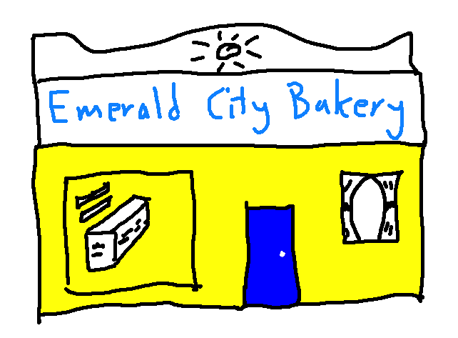
We're broadcasting live from the Emerald City Bakery.
What muffins are for sale today?
Depending on the day, the bakery offers muffins with a variety of add-ons. The set of all possible add-ons is A:
A = {add-ons} = {chocolate-chip, blueberry, orange, almond, lemon, cherry, walnut}
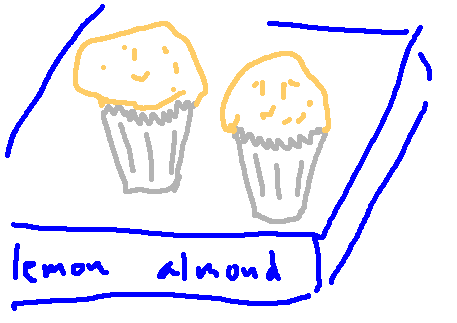
My favorite is their lemon-almond muffin. We can represent this type using the set {lemon, almond}. They also persist in offering cherry-walnut muffins, despite the fact that they seem to be unpopular. I always seem them for sale at deep discount the next day. We can represent this type as {cherry, walnut}.
There could be muffins with one or three add-ons. (I don't think I've ever seen more than three.) For example, {chocolate-chip} or {orange} or {orange, lemon, blueberry}. We represent the one-element muffins as sets for consistency: each type of muffin is represented by a set of add-ons, i.e. a subset of A.
And naturally they offer plain muffins, which can be represented using the empty set \(\emptyset\).
We can now set up a set M that represents all eight types of muffins for sale today.
M = {\(\emptyset\), {orange}, {lemon}, {chocolate-chip}, {lemon, almond}, {cherry, walnut}, {orange, chocolate-chip}, {orange, lemon, blueberry}}
It would be very bad to flatten out the structure to produce something like this:
(NO NO NO!) M = {orange, lemon, chocolate-chip, almond, cherry, walnut, blueberry}
We need the substructure because each element of M is representing a specific type of muffin.
Suppose S is a set. Then the power set of A (shorthand: \(\mathbb{P}(S)\)) contains all subsets of S. For our example set A, \(\mathbb{P}(A)\) is a bit large to write out completely. Here's a partial display of what's in it:
\(\mathbb{P}(A)\) ={\(\emptyset\),
{orange}, {lemon}, ...
{orange, lemon}, {orange, blueberry}, ..., {lemon, blueberry}, ....
{orange, lemon, blueberry}, {orange, lemon, walnut}, ...
{orange, lemon, blueberry, walnut}, ...
....
{chocolate-chip, blueberry, orange, almond, lemon, cherry, walnut}}
To create a subset of A, we have 7 independent two-way choices, one for each flavoring in A. Do we include the flavoring or leave it out? So the power set of A contains \(2^7\) different subsets.
Let's compare \(\mathbb{P}(A)\) and M. \(\mathbb{P}(A)\) contains ALL subsets of A. M contains eight subsets of A. M is a subset of \(\mathbb{P}(A)\).
Remember that the Emerald City Bakery makes muffins with various combinations of these add-ons:
A = {add-ons} = {chocolate-chip, blueberry, orange, almond, lemon, cherry, walnut}
As we just saw, there are \(2^7\) different subsets of A. This count includes the empty set and also the entire set A.
Suppose we ask a different question: how many subsets of A are there containing exactly 3 elements? Recall from the textbook that this is \({7 \choose 3} = \frac{7!}{3!4!}\). To understand this formula, remember that there are $\frac{7!}{4!} = 7\cdot 6 \cdot 5$ ordered lists of 3 objects chosen from a set of 7 objects. But then subsets don't care about the order of their elements. So we divide by $3!$ ways to re-order the three objects.
In general, if our set contains n objects and we wish to pick a subset of size k, the number of possible subsets is \({n \choose k} = \frac{n!}{k!(n-k)!}\).
Now, let's change the problem a bit. Suppose the bakery made 5 types today: plain (p), blueberry (b), cherry (c), orange (o), lemon-almond (L). How many ways can I choose an assortment of 10 muffins for my group meeting?
Notice that the assortment doesn't have an order. So it's like a set, except that we can have more than one copy of some (or all) types. Here are three ways that I might choose the muffins in order. Notice that two of them are the same assortment.
If you haven't seen this sort of problem before, it's not at all obvious how to count the possibilities. If you consider your options for picking each muffin, in order, it's not obvious how to avoid counting the same assortment more than once. There's a trick. And this specific formula is much easier to remember and apply correctly if you know how to derive it.
The first step is to put our muffin types in a specific order. We'll pick this order: p, b, c, o, L. So our three assortments look like this:
Then we're going to put dividers between the types of muffins. We're going to do this like the compartments in a cash register: each type has its own bin, so the dividers stay even if a bin is empty.
Now notice that the letters are redundant. We have a fixed convention about which bin contains which type of muffin. So we can simplify our representations to use a single symbol for each muffin.
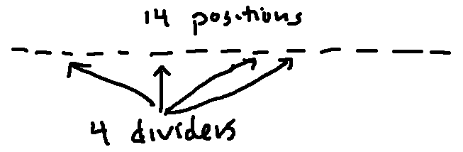
Notice that the dividers can be on the ends. For example, here's how to represent four blueberry, two cherry, and four orange.
| * * * * | * * | * * * *|
Now we have representations that we can easily count. Each one contains 14 symbols: 10 muffins and 4 dividers. The symbols can be arranged in any order. So, to count the possibilities, we have 14 positions, from which we need to choose four to contain the dividers. So we have \({14 \choose 4} = \frac{14}{4! 10!}\) possible assortments.
Notice that we can also count the possibilities by asking how many ways we can choose a set of 10 positions to contain the muffins. So then we have \({14 \choose 10}\) possibilities. But notice that \({14 \choose 10} = \frac{14!}{4! 10!} = {14 \choose 4}\). So both ways to see the problem give us the same answer.
In general, let's suppose that we have n types of muffins and we'd like to choose an assortment of k muffins. Then the formula is \[{{k+(n-1)} \choose {n-1}} = {{k+(n-1)} \choose {k}} \]
As you can see, this formula is a bit difficult to remember. Also, it's extremely easy to get n and k confused. So it is much better to quickly talk yourself through the key points of the construction we just saw: how many objects, how many dividers (which is one less than the number of types).
Here's a picture of one standard graph, called the complete bipartite graph between
2 nodes and 3 notes (shorthand \(K_{2,3}\)).
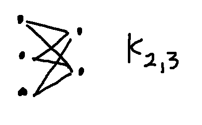
But the two pictures below
are also \(K_{2,3}\). The nodes are color-coded so you can see
which belong to the set of 2 and which to the set of 3.
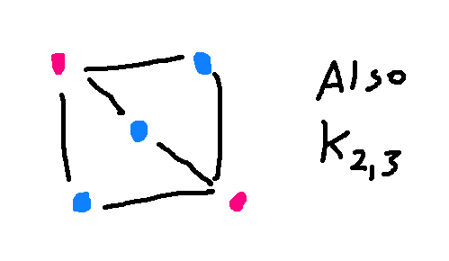
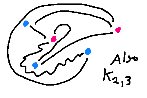
A graph is defined by the nodes and how they are connected. The positions of nodes and the shapes of the edges don't matter mathematically, though obviously some drawings are easier for people to interpret.
The textbook has more details including some other special named graphs.
To show that two graphs have the same structure ("are isomorphic"), you need to
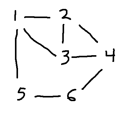
Consider the following two graphs. To line them up, notice that E and 4 are the only nodes with four edges coming into them. So they have to match. Then D has to match to either 6 or 5. Let's pick 6. Since A is directly connected to D and E, we must pair it with 3, otherwise the edges won't match.
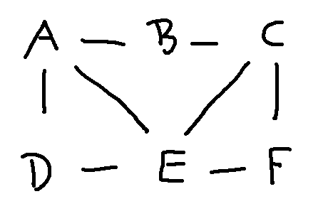
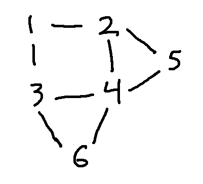
Here's a full matching of the nodes:
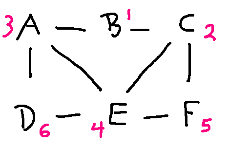
You could also write this out as a table. Unless the graph is complicated, we would usually leave it to the reader (or their computer program) to confirm that the edges line up properly.
| left graph | right graph |
|---|---|
| A | 3 |
| B | 1 |
| C | 2 |
| D | 6 |
| E | 4 |
| F | 5 |
Look at the following graphs. Are they isomorphic? If you fiddle around trying to line them up, it seems like they probably aren't. But how to make a convincing argument?
To show that two graphs are not isomorphic, we need to look at invariant properties, i.e. properties that should be preserved by the matching. That is, we need to look at properties that depend only on the nodes and how they are connected.
The two most obvious invariant properties are the number of nodes and the number of edges. Always a good thing to check, since two graphs can't possibly be isomorphic if those don't match. But they match in this example: 6 nodes and 8 edges.
The next easiest thing to check is node degrees, i.e. how many edges go into each node. Corresponding nodes must have the same degree. And, when we start to look at more complex properties, it's helpful to decorate each node with its degree. Let's do that for our two graphs:
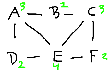
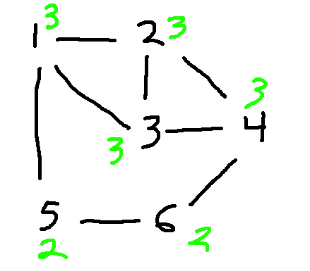
If we list out the node degrees in descending order, we have
Since the degree lists are different, these two graphs aren't isomorphic. In this case, you could make the argument using just one of these degrees: the lefthand graph has a node of degree 4 and the righthand graph doesn't.
Here's another standard graph, called the cycle on 5 nodes (\(C_5\)).
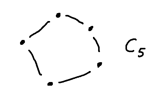
Let add an additional edge between two nodes of $C_5$, to make a graph that I'll call G.
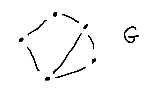
Is G isomorphic to \(K_{2,3}\)?
If we check out the obvious properties, they are the same: 5 nodes, 6 edges, two nodes with degree 3 and three nodes with degree 2. But fiddling around suggests that they don't actually line up.
To show that G and \(K_{2,3}\) aren't isomorphic, we need to find a property that depends only on connectivity and is different for the two graphs. One approach is to look at the two nodes of degree three. There is an edge directly connecting these two nodes in G, but not in \(K_{2,3}\).
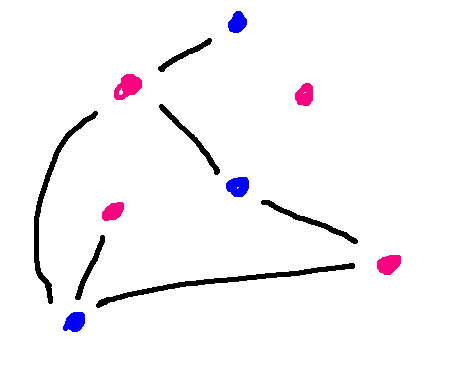
Another approach is to notice that
\(K_{2,3}\) is "bipartite". That is, its nodes can be divided into
two sets, such that all the edges go from one set to the other.
\(K_{2,3}\) is "complete," which means that all possible edges are
actually in the graph. Here's a more typical example of a bipartite
graph, with fewer edges and drawn in a less helpful way. Notice
that all the edges go between a red node and a blue node, never between
two red nodes or two blue nodes.
In a bipartite graph, any walk has to go back and forth between the two sets of nodes. So if the walk needs to end where it started (e.g. a cycle), then it must have an even number of edges. If you look back at our example graph G, it has a 5-cycle. Since \(K_{2,3}\) is bipartite, it cannot have a 5-cycle. That's another way to argue that these two graphs aren't isomorphic.
We've seen a range of connectivity-based features that can be compared between two graphs, to show that they aren't isomorphic.
If we run out of clever features to compare, the backup plan is a careful exhaustive search of all ways to line up the nodes. If you ever have to do this, use any available features (esp. node degrees) to limit what possible matches you need to consider for each node.